


Real arithmetic is a case where familiarity breeds contempt. Most of the issues that we need to consider are extremely well known as folklore, but we do not know of a published account that considers them all and gives the details in a coherent form that is suitable for us. See [TvD88, p260] for a metrical approach involving 2−n, but our paper is about Dedekind cuts and intervals, which are fundamentally order-theoretic ideas.
Dedekind himself considered addition and square roots but not multiplication [Ded72]. Even in the classical situation, the proof that the positive and negative reals form a commutative ring or field involves either an explosion of cases or considerable ingenuity. One ingenious solution is John Conway’s definition of multiplication [Con76, pp.19–20], but we shall not use it.
Working with intervals instead of numbers makes this problem worse, whilst its usual solution — case splitting — is unacceptable, at least for R, in constructive analysis [TvD88, §5.6], topos theory [FH79] [Joh77, §6.6] or ASD.
On the positive side, general continuity will relieve us of the burden of checking the arithmetic laws, and in particular the case analysis in R. However, (Scott) continuity is only applicable after we have verified an order-theoretic property of discrete rational arithmetic (cf. Proposition 7.13). In Q we can and do use case analysis.
For reasons of space we omit the multiplication sign (×) in the usual way. Juxtaposition may therefore denote either multiplication or function application, but our alphabetic conventions distinguish them: a b with two italic letters is multiplication, whilst φ a with a Greek letter is application. Despite the weight of tradition, we use p instead of є for a small positive tolerance, saving (δ,υ) and (є,τ) for the arguments of an arithmetic operation on cuts, with result (α,σ).
As usual, multiplication and λ-application bind more tightly than <, which is tighter than ∧ .
Axiom 11.1 Q is a discrete, densely linearly ordered
(Definition 6.1) commutative ring.
There is a unique “inclusion” map ℤ⊂ Q
that preserves and reflects =, <, 0, 1, +, − and ×.
Axiom 11.2
Q obeys the Archimedean principle, for p,q:Q,
| q> 0 =⇒ ∃ n:ℤ. q(n−1) < p< q(n+1). |
In view of Proposition 6.5, this cannot be a property of the order (Q,<) alone: it says how ℤ (i.e. the additive subgroup generated by q) lies within the order. We isolate our use of this principle in Propositions 11.15 and 12.7, in the hope that some future development may avoid it altogether (Remark 12.13).
Remark 11.3 We do not ask that Q be a field, with (exact) division,
because we have in mind the ways in which
it might be represented computationally: the axioms
ought at least to allow the dyadic and decimal rationals as examples.
We could weaken the properties of addition and multiplication on Q
still further,
since (in Example 11.9 and Proposition 12.3)
we shall only use them in the form of the four ternary relations
| a< d+e u+t< z a< d× u u× t< z, |
whose axiomatisation we leave to the interested reader. Such a person may be an interval analyst or programmer who wants to use ASD to obtain mathematically provable results from the floating point arithmetic that is built in to computer hardware [Ste85].
Whilst the likely applications have it, we do not actually even need to assert division by 2 as an axiom:
Lemma 11.4 There is an approximate half,
h:Q, with 0< h+h< 1.
Proof Let a,h:Q with 0< a< 1 and 0< h<min(a,1−a). ▫
Since the operations of arithmetic take two arguments, and its equations involve (up to) three variables, our first task is to define the objects R2 and R3. By Rn here we simply mean the product of 2, 3, … copies.
Proposition 11.5 The product spaces Rn exist,
and they are overt, with ∃Rn=∃Qn.
Proof Axiom 4.1 gives product types, and by Lemma 9.1 the quantifiers are given by
|
Remark 11.6 Now we have a diagram that combines those in Remarks
2.13 and 6.9,
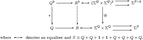
This means that a term of type R2 is a pair of solutions of equations, defining a pair of cuts or a “Dedekind cross-hair”, i.e. a division of the rational plane into quadrants. R2 is, in fact, a Σ-split subspace [B], though the splitting I2 is not simply the square of that for R. But that does not matter, as we shall not need it anyway.
Exercise 11.7 By analogy with Proposition 2.15, find
I2:ΣR× R↣ΣΣQ×ΣQ×ΣQ×ΣQ.
Remark 11.8
The plan, for each arithmetic operation ∗ (+ or ×), is
| (δq,υq)⊛(δr,υr) = (δq∗ r,υq∗ r):ΣQ×ΣQ; |
Classically, Ramon Moore has already done the first of these tasks, but we need to take account of the more general intervals that exist constructively (Remarks 2.3f). Recall from Propositions 7.12f that the intervals with (rational) endpoints provide a basis in the sense of domain theory, and that we may extend a predicate φ(d,u) to Φ(δ,υ) such that Φ(δd,υu)⇔φ(d,u) so long as φ is rounded, in the sense that
| φ(e,t) ⇔ ∃ d u.(d< e)∧(t< u)∧φ(d,u). |
This condition may easily be generalised to an n-ary operation, but that would lead to another explosion of symbols and cases. It is therefore wise to consider the arguments and the bounds one at a time, which is enough.
Example 11.9 Consider the bounds a,z on addition
of a fixed rational interval [e,t], so
| φ(d,u) ≡ a< [d,u]⊕[e,t]< z ≡ a< d+e ∧ u+t< z. |
Then this condition requires a< d+e ⇔ ∃ d′. (d′< d)∧ (a< d′+e), for which we choose d′ with a−e< d′< d, using subtraction and interpolation, and similarly for the upper bound. ▫
Notation 11.10
For (δ,υ),(є,τ):ΣQ×ΣQ, let
| (δ,υ) ⊕ (є,τ) ≡ (λ a.∃ d e.(a< d+e) ∧δ d∧є e, λ z.∃ u t.(u+t< z)∧ υ u∧τ t). |
Remark 11.11
It’s worth spelling out the condition in Proposition 7.13
once more in interval notation.
Write x for (the name of) an interval with rational endpoints
[x,x], and
| x⋐y ≡ [ |
| , |
| ]⊂ ( |
| , |
| ) ≡ |
| < |
| ∧ |
| < |
|
for the strict containment relation that relates the basic compact subspace [x,x] to the basic open one (y,y), cf. [K]. (Beware that ⋐ corresponds to ≫ in the bounded interval predomain IR, which is a continuous dcpo.) Then the condition for ⊛ to be well defined is
| x⊛y⋐w ⇔ ∃x′y′. x⋐x′ ∧ y⋐y′ ∧ x′⊛y′⋐w. |
Note that ∃ here ranges over the names of the intervals, i.e. over {(d,u) ∣ d≤ u}⊂ Q2, which is a discrete space, not over the domain IR, since ⋐ is not defined there as an ASD predicate in the sense of Axiom 4.2, but see Section G 11.
Since it is only required to compute x⊛y to the limited precision w, it is standard programming practice to use less precise versions x′ and y′ of x and y in this way, thereby saving space and hence time.
Using roundedness, Proposition 7.12 extends Moore’s operations to general intervals by
| (δ,υ)⊛(є,τ) ≡ (α,σ), where α |
| ∧σ |
| ≡ ∃xy.δ |
| ∧υ |
| ∧є |
| ∧τ |
| ∧x⊛y⋐w. |
Turning to stage (b) of the plan in Remark 11.8, we have to check that each formula that we introduce for an operation actually gives rounded, bounded, disjoint and located pairs (α,σ). Roundedness and boundedness follow immediately from the form of the definition that we have just given. We also get disjointness for free:
Lemma 11.12
Let α,σ:Rn⇉ΣQ be
“disjoint” on Qn, in the sense that
| a,z:Q, |
| :Qn ⊢ α |
| a∧(z< a)∧σ |
| z ⇒ ⊥. |
Then they are also disjoint on Rn in the same sense, cf. Proposition 9.5.
Proof By Proposition 11.5, αx a∧(z< a)∧σx z ⇒ ∃ q.αq a∧(z< a)∧σq z ⇒ ⊥. ▫
Lemma 11.13
Addition (Notation 11.10) takes intervals
(i.e. rounded, bounded and disjoint pseudo-cuts) to intervals,
⊕:IR× IR→ IR.
Proof (δ,υ) ⊕ (є,τ) is rounded by transitivity and interpolation in (Q,<), keeping the same d,e,u,t. It is bounded because (δ,υ) and (є,τ) are bounded, and by extrapolation in (Q,<). It is disjoint by the previous Lemma, but more directly,
|
since u+t< d+e⇔(u−d)+(t−e)< 0⇒(u< d)∨(t< e). ▫
Remark 11.14 Locatedness always seems to be the most difficult step,
because we need to calculate the result arbitrarily closely.
Recall that we defined this in a purely order-theoretic way in
Definition 6.8, namely d< u⇒δ d∨υ u.
However, to prove this property of a sum, we shall need a stronger hypothesis on the summands. This is actually the version of locatedness that most accounts of Dedekind cuts use, except that we allow the tolerance p to be any positive element of Q, not just 2−n for n:ℕ.
It is not difficult to see the necessity of the stronger hypothesis for what we’re trying to achieve, namely that Q is to be dense in a Dedekind-complete Abelian group R. In this situation, for any x≡(δ,υ):R, there must be d,u:Q with x−½ p< d< x< u< x+½ p. This is the (apparently essential) use of the Archimedean principle, to which we shall return in Remark 12.12.
Proposition 11.15 Any cut (δ,υ)
is arithmetically located, i.e. for p:Q,
| p> 0 =⇒ ∃ e t:Q.δ e∧υ t∧ (0< t−e< p). |
Conversely, if (δ,υ) is rounded and arithmetically located then it is bounded and located.
Proof By boundedness, δ d∧υ u for some d< u:Q. Then the Archimedean principle gives some k:ℕ with u−d< k h p, where 0< h+h< 1 by Lemma 11.4. So qj≡ d + j hp satisfy
| q0≡ d< q1< q2<⋯< qk−1< qk > u, |
to which we may apply Lemma 6.16, as (δ,υ) is order-located with δ q0 and υ qk. This gives δ e∧υ t∧ (t−e< p), where e≡ qj, t≡ qj+2 and t−e=2 h p< p, for some 0≤ j≤ k−2.
Conversely, given d< u, let e,t:Q with t−e< u−d such that δ e, υ t, so (δ,υ) are bounded. By locatedness of < (Lemma 6.2), e< d∨ t< u, so δ d∨υ u by roundedness. ▫
Lemma 11.16 Addition takes cuts to cuts.
Proof Given a< z, we use arithmetic locatedness of one summand, (δ,υ), with p≡ z−a, to give d,u:Q such that δ d, υ u, d< u and (u−d)<(z−a). Since a−d< z−u, by interpolation there are e,t:Q with a−d< e< t< z−u, so a< d+e and u+t< z. By order locatedness of the other summand, є e∨τ t, so we have shown that
| ∃ d e u t:Q. (a< d+e) ∧ δ d ∧ (є e∨τ t) ∧ (u+t< z) ∧ υ u. |
This implies that (α,σ) is order-located, i.e.
| (∃ d e. (a< d+e) ∧ δ d∧ є e) ∨ (∃ u t. (u+t< z) ∧ υ u ∧τ t). ▫ |
Exercise 11.17 Show directly that
In the final step (c) of Remark 11.8, topology plays to our advantage, particularly in ASD, where all definable maps are automatically continuous. Once we have thought of a definition for the extended operations, and verified that they have real results (i.e. cuts), the laws of arithmetic (both equations and inequalities) transfer automatically from Qn to Rn.
| if |
| :Qn⊢ f( |
| )≤ g( |
| ):R then |
| :Rn⊢ f( |
| )≤ g( |
| ):R. |
Proof In traditional notation, since R is Hausdorff and f,g are continuous, the subspace
| C ≡ |
| ⊂ Rn |
on which the laws actually hold is closed; on the other hand, Qn⊂ Rn is dense, whilst Qn⊂ C by hypothesis, so C=Rn. In ASD, C is co-classified by θ, where
| θ( |
| ) ≡ f( |
| )> g( |
| ), and θ( |
| ) ⇒ ∃ |
| .θ( |
| ) ⇔ ⊥ |
by Proposition 11.5, so θ=⊥. ▫
Proposition 11.19 R is an ordered Abelian group. ▫