


We begin by recalling Richard Dedekind’s construction, and relating it to some ideas in interval analysis. These provide the classical background to our abstract construction of R in ASD, which will start with our formulation of Dedekind cuts in Section 6. In this section we shall use the Heine–Borel theorem to prove an abstract property of ℝ, from which we deduce the fundamental theorem of interval analysis. The same abstract property, taken as an axiom, will be the basis of our construction of R and proof of the Heine–Borel theorem in ASD.
Remark 2.1 Dedekind [Ded72]
represented each real number a∈ℝ
as a pair of sets of rationals,
{d ∣ d≤ a} and {u ∣ a< u}.
This asymmetry is messy, even in a classical treatment,
so it is better to use the strict inequality in both cases,
omitting a itself if it’s rational.
So we write
| Da ≡ {d∈ℚ ∣ d< a} and Ua ≡ {u∈ℚ ∣ a< u}. |
These are disjoint inhabited open subsets that “almost touch” in the sense that
| d< u =⇒ d∈ D ∨ u∈ U. |
This property is usually known as locatedness.
The idea that a set of rationals is open in the usual topology on ℝ and extends towards ±∞ can be expressed order-theoretically, using a condition that we shall call roundedness:
| d∈ D ⇔ ∃ e.d< e∧ e∈ D and u∈ U ⇔ ∃ t.t< u∧ t∈ U. |
A real number represented as a cut is therefore a pair of subsets, i.e. an element of ℘(ℚ)×℘(ℚ), that is rounded, bounded (i.e. inhabited), disjoint and located.
Exercise 2.2 If Δ⊂ℝ is an open set of
reals that extends downwards, show that D≡Δ∩ℚ is a
rounded set of rationals with the same property, and that this defines
a bijection between such subsets, where
Δ≡{r∈ℝ ∣ ∃ q∈ D.r< q}.
In future we shall write D for either representation,
and pass between them without comment;
in particular, in “ℝ∖(D∪ U)” below,
real as well as rational numbers are removed.
Definition 2.3
It is very useful to generalise the notion of Dedekind cut
by dropping the locatedness condition.
Instead of almost touching,
and so representing a single real number a∈ℝ,
such a pseudo-cut corresponds classically to
a closed interval [d,u]≡ℝ∖(D∪ U).
We sometimes weaken the other conditions too,
allowing D≡∅ and d≡−∞,
or U≡∅ and u≡+∞.
The extension of the arithmetic operations to such intervals was defined by Ramon Moore [Moo66]:
|
The formula for multiplication is complicated by the need to consider all possible combinations of signs.
Remark 2.4
Moore’s interval analysis has been used to develop a
variety of numerical algorithms; see [Kea96]
for a brief survey with an extensive bibliography.
Amongst these, we focus on what it achieves for the problem of
optimisation.
By this, we understand finding the maximum value
of a continuous function defined on a non-empty compact domain,
but not necessarily any location where the function attains that value.
Plainly, any value of the function provides a lower bound
for the maximum, but finding upper bounds is problematic
using standard numerical methods, especially when the function has “spikes”.
For the sake of illustration, consider an arithmetical function f:[0,1]n→ℝ. If this is just addition or multiplication, Moore’s interval operations provide the minimum and maximum values of the function on the domain directly. For a more complicated arithmetical function, we interpret the operations according to Moore’s formulae, and may (if we’re lucky) still obtain the minimum and maximum.
In general, however, the result of Moore’s interpretation will be an interval that contains the required image. In other words, it provides an upper bound of the maximum — exactly what standard numerical methods find difficult. Unfortunately, this may be a vast over-estimate, especially when the definition of the function is complicated and involves subtraction of similar large numbers, so this does not really help very much with spiky functions.
In fact, Moore and his followers have provided various techniques for reducing the sizes of the resulting intervals. One of these simply massages the arithmetic expression to reduce multiple occurrences of variables and sub-expressions, since computing x−x introduces a large error that can easily be avoided. However, these techniques are not the purpose of the present discussion.
Remark 2.5 We regard Moore’s definitions as merely
one way of extending certain continuous functions
to take intervals instead of real numbers as arguments.
In fact, that’s exactly the point:
| F0[d,u] ≡ {f x ∣ x∈ [d,u]}, |
| F[a,a] = [f a,f a] and F0[d,u]⊂ F[d,u]. |
Whilst Moore’s interpretation may give a huge over-estimate of the image if we don’t rewrite the expression, it has an important technical property, namely that it preserves (syntactic) composition of arithmetic expressions, so it is easily performed by a compiler.
The first question that this raises is whether the ideal operation F0, which (a) defines set-theoretically, is continuous. Then we can ask whether there is a way of computing it, using (b).
Continuity is crucial to our whole development: not only that of the single operation F0, but also for the process that extends f to F or F0. However, as ℘(ℚ) is a complete lattice, rather than a space that has a familiar Hausdorff topology motivated by geometry, we first have to describe what its topology is. (In this paper, we do not even attempt to put a topology on ℝℝ.)
Definition 2.6
Let L be a complete lattice such as ℘(ℚ).
Then a family U⊂ L is called Scott open
[Sco72a, GHK++80] if it is
This Scott topology is never Hausdorff (except, that is, on the trivial lattice).
A function f:L1→ L2 between complete lattices is continuous with respect to the Scott topology iff it preserves directed unions. In particular, it is monotone, i.e. if x⊑ y in L1 then f x⊑ f y in L2. See Section J 3 for a brief account of this topology that is enough for its use here.
Exercise 2.7
Let L be the topology (lattice of open subsets) of any
topological space X, and K⊂ X any subset.
Show that the family U≡{U ∣ K⊂ U} of
open neighbourhoods of K is Scott open iff K is compact
in the usual “finite open sub-cover” sense.
If this is new to you, you would be well advised to stop
at this point to see for yourself why this is the case,
since this idea is fundamental to our whole programme. ▫
Example 2.8
Let L≡ℝ≡ℝ+{−∞,+∞},
considered as a complete lattice in the arithmetical order,
so +∞ is the top element.
Equipped with the Scott topology, this space arises in real analysis
because lower semicontinuous functions X→ℝ
are just functions X→ℝ that are continuous
in the sense of general topology.
We shall see, however, that it is a mistake to think of ℝ
as derived from ℝ in this clumsy way:
it is really simpler and more fundamental than ℝ itself.
Its elements, which we call ascending reals,
are given by Exercise 2.2,
i.e. in a similar way to the Dedekind reals,
except that only the lower cut D⊂ℚ is used.
The descending reals, ℝ,
are defined in the same way, but with the opposite order,
and are related to upper semicontinuous functions.
The words “ascending” and “descending” relate the usual temporal
language about the real line to the vertical intuition of lattice theory.
▫
Remark 2.9
It is useful theoretically to consider more general intervals
than Moore did, i.e. not necessarily having rational endpoints.
For example, a computation that is allowed to continue forever
may generate a converging pair of sequences of rationals,
| d0 < d1< d2< ⋯ < u2 < u1 < u0, |
whose limits supdn and infun we would like to see as the ‘ultimate result’ of the computation.
If these limits exist in ℝ, say d≡supdn and u≡infun, then [d,u] is the (directed) intersection ⋂[dn,un]. However, d and u are best seen as ascending and descending reals,
| D ≡ {d ∣ ∃ n.d< dn}∈ |
| and U ≡ {u ∣ ∃ n.u> un}∈ |
| , |
since, constructively, they need not exist as members of the usual “Euclidean” structure (Remark 15.1). Nevertheless, the intersection of the closed intervals does exist: it is ℝ∖(D∪ U), and is always a closed subspace.
Notice that the open subsets D and U represent positive information, namely the lower and upper bounds that we have verified so far for the real number that we’re trying to calculate. The closed interval [d,u], on the other hand, consists of the candidate real numbers that we have not yet excluded, which is negative information.
Definition 2.10 We can consider these generalised intervals as members
of the interval domain, Iℝ [Sco72b, ES98].
The order relation is traditionally defined as reverse inclusion
of closed intervals, and so directed joins are given by intersection.
According to our preferred view, an interval is defined as a generalised Dedekind cut (D,U), and the order relation is the forward inclusion of these sets. As we acquire more information about the number, in the form of tighter bounds, the correspondingly narrowing interval goes up in the order on the domain.
We shall now start using some of the notation of the calculus that we intend to introduce.
Notation 2.11
Classically, any subset D⊂ℚ may be represented as a function
ℚ→{⊤,⊥} that says whether or not each d∈ℚ
belongs to D.
Since we believe that topology is fundamental,
we give this target set the Scott topology.
It then becomes the Sierpiński space,
in which just one singleton {⊤} is open,
making the other {⊥} closed.
It therefore looks like
| , |
and we shall call it Σ.
Since ℚ is discrete, it doesn’t change much to require our functions ℚ→Σ to be continuous. However, for a general topological space X (such as ℝ), continuous functions φ:X→Σ correspond bijectively to open subspaces U⊂ X, by U≡φ−1(⊤). We shall say that φ classifies U.
Notation 2.12
Having passed from the (open) subset D⊂ℚ
to a (continuous) function δ:ℚ→Σ,
we also replace set-theoretic notation with the λ-calculus.
A function x↦φ(x) is written as a λ-abstraction
λ x.φ(x);
we use nested λ-abstractions for several variables,
but write λ x y.σ instead of λ x.λ y.σ.
Application φ(a) is written without parentheses, φ a.
Expressions built from λ-abstractions and applications
are called λ-terms.
So in ASD we represent D and U by λ-terms δ,υ:Σℚ, adopting the convention of using Greek letters for terms of this type. Many authors in computer science would write ℚ→Σ instead of Σℚ, which is the notation in pure mathematics. Membership d∈ D is written δ d, and set-formation becomes λ-abstraction. In particular, Da and Ua become
| δa ≡ λ d.(d< a) and υa ≡ λ u.(a< u), |
so δa d means d< a. Then any real number can be represented as a pair (δ,υ) of λ-terms, and the real line as a whole is a subset ℝ⊂Σℚ×Σℚ.
Remark 2.13
We want to use this representation to compute with real numbers,
and in the first instance to do arithmetic with them.
Dedekind indicated how this can be done, defining operations on cuts.
But there is a difference between his objective of providing
a rigorous foundation for differential and integral calculus,
and ours of getting a machine to compute with real numbers.
He only had to define and justify the operations on legitimate cuts
(those that are rounded, bounded, disjoint and located),
whereas our machine will do something with any pair
of λ-terms that we give it,
even if that’s only to print an error message.
It’s reasonable to ask that any program F that is intended to compute a function f:ℝ→ℝ using Dedekind cuts will actually take any pair of λ-terms and return another such pair. We say that the program is correct for this task if, when it is given the pair (δa,υa) that represents a number a, it returns the pair (δf a,υf a) that represents the value f(a) of the function at that input. In other words, the square on the left commutes:
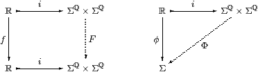
Remark 2.14
We shall not attack the problem of extending functions directly.
It is simpler and more in keeping with the ideas of computation,
Dedekind cuts and topology to consider first how
an open subset of ℝ may be extended to one of Σℚ×Σℚ.
Recall from Notation 2.11 that such an open subset is classified by a continuous function taking values in Σ. We expect the function φ from ℝ (classifying an open subset of it) to be the restriction of a function Φ from Σℚ×Σℚ (classifying an open subset of that), making the triangle on the right above commute. In other words, ℝ should carry the subspace topology inherited from the ambient space, Σℚ×Σℚ, which itself carries the Scott topology.
This extension of open subspaces is actually the fundamental task, since we can use it to extend functions by defining
| F(δ,υ) ≡ (λ d.Φd(δ,υ), λ u.Ψu(δ,υ)), |
where Φd and Ψu are the extensions of φd≡λ x.(d< f x) and ψu≡λ x.(f x< u) respectively.
The extension process must therefore respect parameters. We implement this idea by introducing a new operation I that extends φ to Φ in a continuous, uniform way, instead of a merely existential property of the extension of functions or open subspaces one at a time. This depends on an understanding of Scott-continuous functions of higher type.
Proposition 2.15
Classically, there is a map I:Σℝ↣ΣΣℚ×Σℚ, defined by
| (V⊂ℝ) open ↦ {(D,U) ∣ ∃ d∈ D.∃ u∈ U.(d< u)∧[d,u]⊂ V} |
in traditional notation, or
| φ:Σℝ↦ λδυ.∃ d u. δ d∧υ u∧(d< u)∧∀ x:[d,u].φ x |
in our λ-calculus, that is Scott-continuous. It makes Σℝ a retract of ΣΣℚ×Σℚ, as it satisfies the equation
| Σi· I = idΣℝ or x:ℝ, φ:Σℝ ⊢ Iφ(i x) ⇔ φ x, |
where i x≡(δx,υx):Σℚ×Σℚ. This expresses local compactness of ℝ.
Proof The Heine–Borel theorem, i.e. the “finite open sub-cover” definition of compactness for the closed interval [d,u], says exactly that the expression “[d,u]⊂ V” is a Scott-continuous predicate in the variable V:Σℝ (Exercise 2.7). Thus the whole expression for I is a Scott-continuous function of V. This satisfies the equation because, if φ classifies V⊂ X,
| φ a ≡ (a∈ V) ↦ Iφ(i a) ≡ (∃ d u. a∈(d,u)⊂ [d,u]⊂ V) ⇔ (a∈ V). ▫ |
The argument so far has relied on the prior existence of ℝ. The next step is to eliminate real numbers in favour of rational ones.
Lemma 2.16
Since Φ:Σℚ×Σℚ→Σ is a Scott-continuous function,
|
where pk≡ d+2−m k (u−d), for any chosen d< u. Although pk also depends on m, d and u, we omit them to simplify the notation: they should be understood to come from the expression in which pk is embedded.
Proof In traditional notation, the unions
| Df = ⋃e< f↑ De and Us = ⋃s< t↑ Ut |
are directed, cf. Remark 2.9, so Φ preserves them. The equations above say the same thing in our λ-calculus (Notation 2.12). Notice that (⇐) is monotonicity. Having enclosed the point x in some open interval (e,t), we may find m and k so that e< pk−1< x< pk+1< t. ▫
Proposition 2.17
The idempotent E≡ I·Σi on ΣΣℚ×Σℚ is given by
| E Φ (δ, υ) ≡ ∃ n≥ 1. ∃ q0 < ⋯ < qn. δ q0 ∧ υ qn ∧ ⋀k=0n−1 Φ(δqk, υqk+1). |
Proof Substituting i x≡(δx,υx) into the definition of I in Proposition 2.15,
| (I·Σi)Φ (δ,υ) ≡ I(λ x.Φ (i x)) (δ,υ) ≡ ∃ d u. δ d∧υ u∧(d< u)∧ ∀ x:[d,u].Φ(δx,υx). |
[E⊑ I·Σi]: Although the formula for E essentially involves abutting closed intervals,
| [d,u] = [q0,q1]⋃[q1,q2]⋃⋯⋃[qn−1,qn], |
part (a,⇒) of Lemma 2.16 expands each of them slightly, from [qk,qk+1] to [e,t]. Then each x∈[d,u] lies inside one of the overlapping open intervals (e,t):
|
where the last step uses Lemma 2.16(a,⇐) with f≡ s≡ x.
[E⊒ I·Σi]:
For the converse, Lemma 2.16(b,⇒)
also encloses each point x∈[d,u] in an open interval
(pk−1,pk+1)∋ x with dyadic endpoints,
such that Φ(pk−1,pk+1) holds.
Although some points x may â priori
need narrower intervals than others, with larger values of m,
the Heine–Borel theorem says that finitely many of them suffice,
so there is a single number m that serves for all x∈[d,u].
Another way of saying this is that the universal quantifier ∀ x:[d,u]
is Scott-continuous, preserving the directed join ∃ m.
|
where we trim the intervals using Lemma 2.16(a,⇒) and omit the last one. Then n≡ 2m, q0≡ p0≡ d, q1≡ p1, …, qn≡ p2m≡ u provide a sequence to justify EΦ(δ,υ). ▫
Remark 2.18
Notice that this formula for E
involves only rational numbers (and predicates on them) but not reals.
We can write this formula with very little assumption about
the underlying logic.
The role of the classical Heine–Borel theorem was to define a different map,
I, to prove that it is Scott-continuous and that it satisfies the equations
| Σi· I = idΣℝ and I·Σi = E. |
It is the formula E — not the classically defined map I or the accompanying proof — that we shall use to construct the real line in ASD. In Section 15 we shall discuss some systems of analysis in which the Heine–Borel theorem fails, and the operation I does not exist either.
Besides the construction of R in ASD, the formula is important for many other reasons. In particular, it shows how Moore’s interval arithmetic solves the optimisation problem, and justifies the interval-subdivision algorithms that have been developed using interval analysis. It would be appropriate to call it the fundamental theorem of interval analysis. Moore himself proved it [Moo66, Chapter 4] using convergence with respect to the metric
| ∂([d,u],[e,t]) ≡ max(|d−e|,|u−t|). |
Corollary 2.19
Let f:ℝ→ℝ be a continuous function
and F be any continuous extension of f to intervals
(Remark 2.13).
For example, if f is an arithmetic expression then F may be
its interpretation using Moore’s operations.
Suppose that e and t are strict bounds for the image of [d,u] under f,
so
| ∀ x:[d,u].e< f x< t, or, equivalently, F0[d,u] ⊂ (e,t), |
where F0 gives the set-theoretic image. Then there is some finite sub-division (which could be chosen to be dyadic), d≡ q0< q1<⋯< qn−1< qn≡ u, such that
| (e,t) ⊃ ⋃m=0n−1 F[qk,qk+1]. |
Moreover, we obtain F0 from F in Remark 2.5 using E and Remark 2.14. ▫
This sub-division could be found by a recursive program that either applies the function Moore-wise to the whole interval, or splits it and calls itself on each half.
Remark 2.20
Finally, some curious things happen in both interval analysis
and ASD when we play around with the formulae.
Of course, if a< b then the subsets
| D≡ Db≡{d ∣ d< b} and U≡ Ua≡{u ∣ a< u} |
overlap. But we may still apply Proposition 2.15 to them, obtaining the existential quantifier,
| (Db,Ua)∈ I V ⇔ ∃ x:[a,b].x∈ V. |
We shall see in Section 10 that both quantifiers are derived from E like this.
Given that ∀ is related to overestimation of the range of a function in interval analysis, could this back-to-front version for ∃ yield an underestimate? It is obviously very dangerous in this case to rely on any intuition of an interval as a single closed set, as is common in the literature on interval analysis. On the other hand, there is no problem in dealing with a back-to-front interval in our formulation of it as a pair (D,U) of (now overlapping) open sets.
In order to exploit this idea, we would have to begin with a careful study of the arithmetic, which was introduced by Edgar Kaucher [Kau80]. Addition and subtraction are as in Remark 2.3, but multiplication is more complicated (Lemma 12.1). Various authors have used Kaucher’s arithmetic to investigate questions of linear algebra, logic and underestimation, e.g. [KNZ96, Lak95].