


Now that the calculus is complete, we can use it to express some familiar ideas in elementary analysis such as continuity, differentiability and Riemann integration.
Remark 10.1
Classically, a point x is said to be in the interior
of a subset U⊂ℝ if x∈(d,u)⊂ U for some d,u:ℝ.
For any d< e< x< t< u, this is equivalent to
| ∃ e t. x∈(e,t)⊂[e,t]⊂(d,u)⊂ U, |
which states local compactness of ℝ (cf. Definition 3.18). This can be formulated in the ASD λ-calculus, because we can use the universal quantifier to say when a closed interval is contained in an open subspace.
Theorem 10.2 Every point a:ℝ
that is a member of the open subspace classified by φ:Σℝ
is in its interior, in the sense that
| φ a ⇔ ∃ d u. (d< a< u) ∧ ∀ k:[d,u].φ k ≡ ∃δ>0.∀ k:[a±δ].φ k. |
Proof This uses the uniformity principle (Corollary 9.4) that we derived from Scott continuity of the universal quantifier. However, since in this case the existentially quantified variable δ is a parameter of the universal quantifier ∀ k:[a±δ] itself, we reformulate the problem, using the directed relation θ(k,δ) ≡ (|k−a|>δ)∨φ k with δ↘ 0. Then
|
Before going on, you should pause to consider what we have done. This statement is not true in set theory, that is, for predicates φ of the logical generality with which you are familiar. We have proved a Theorem that agrees with topology, by devising a logic with axioms that are themselves appropriate to that subject (Remark 5.1).
This also ties up some loose ends in the foundations of ASD:
Corollaries 10.3 For any predicate φ:Σℝ,
Hence, as in Definition 3.3, it doesn’t matter whether we use ℚ or ℝ when we define the ascending or descending reals, or invoking uniformity in Proposition 9.3. Also, Dedekind cuts (Axiom 6.8) may be eliminated in the same way as descriptions (Lemma 6.3).
It’s time to do some basic real analysis, using this key result.
Theorem 10.4
Every function f:ℝ→ℝ
is continuous in the ε–δ sense.
Proof For x:ℝ and ε>0, put φ y ≡ (|f y−f x|<ε). Then Theorem 10.2 provides the input tolerance, but in the form of a closed interval [x±δ] instead of the traditional open one:
| ε> 0 ≡ (|f x−f x|<ε) ≡ φ x ⇔ ∃δ>0.∀ y:[x±δ].φ y, |
so
| ε>0=⇒ ∃δ>0.∀ y:[x±δ]. (|f y−f x|<ε). ▫ |
Remark 10.5 This statement only differs from the familiar one in that
Remark 10.6 Similarly, any function of two variables is jointly continuous
in the sense that
| ε> 0=⇒ ∃δ> 0.∀ x′:[x±δ].∀ y′:[y±δ]. (|f x′ y′−f x y|<ε), |
i.e. with the sup metric on ℝ×ℝ, so its topology Σℝ×ℝ is the usual Tychonov one. ▫
When we want to interchange limiting processes in analysis such as sums of power series, and in integration and differentiation, we know that the δs that they involve have to exist uniformly in the other variables. Uniformity is essentially the ability to interchange quantifiers, as we saw in the previous section. We can use more or less the same argument that we used for continuity to prove the stronger result:
Theorem 10.7 Any function f:ℝ→ℝ is
uniformly continuous on any compact subspace K⊂ℝ.
Proof Consider the predicate x,y:ℝ, ε> 0 ⊢ φ(x,y,ε) ≡ (|f x−f y|<ε) . Then, as before,
| ε> 0 ⇔ φ(x,x,ε) ⇔ ∃δ>0.∀ y:[x±δ].φ(x,y,ε). |
By the same argument as in Theorem 10.2, with δ↘0,
|
Remark 10.8 Here is the translation of our argument into traditional language;
it appears to be essentially the one that G.H. Hardy used
in [Har08, §107].
Our φ classifies
| U ≡ {(x,y) ∣ |f x−f y|<ε} ⊂ K× K. |
This is a neighbourhood of the diagonal, every point of which lies inside an open δ-ball within U. As the diagonal is compact, finitely many such balls suffice to cover it, and we let δ be their minimum size, which is positive.
Another, much more complicated, argument appears in many textbooks, for example [Dug66, Theorem XI 4.5]. The image of the domain K is a compact subspace of the codomain, so finitely many ε-balls cover its image, and their inverse images cover the domain. Now calculate the Lebesgue number, i.e. the size of the smallest non-empty intersection; this is the required δ.
Although the remaining sections of this paper will study continuous functions, we pause to demonstrate how the definitions of differentiation and integration can be stated in our language. The message is that they naturally yield Dedekind cuts rather than Cauchy sequences, whilst uniformity is captured by Corollary 9.4.
Definition 10.9 Many accounts of differentiability
(in my view, the better ones) use the expression
| f(x+h) = f(x) + h f′(x) + o(h) |
instead of the limit of a quotient. Constructive authors have found it most convenient to define the derivative as the pair, (f,f′), rather than f′ alone. In order to give a definition using Dedekind cuts, we must therefore bound both the derivative and the original function,
| e0< f(x)< t0 and e1< f′(x)< t1. |
We can express this using bounds on the function over some interval around x,
|
which confines the function to a region in the shape of a “bow tie”, cf. [EL04, §3.1]:
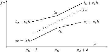
Considered as a predicate in (e0,t0) or (e1,t1), this formula
Differentiability also gives another example of the relationship between the quantifiers and uniformity.
Proposition 10.10
Any function that is differentiable everywhere
in a compact domain K is uniformly differentiable there.
Proof Inside all of the quantifiers in the definition of the derivative above there is a propositional expression φ(x,h) that does not depend on δ. For any such formula, we note that
| (0<δ<δ′) ∧ ∀ h:[0,δ′].φ(x,h) =⇒ ∀ h:[0,δ].φ(x,h), |
simply because of the range of the quantifier ∀ h. Hence, by Corollary 9.4, as δ↘ 0,
| ∀ x:K.∃δ> 0.∀ h:[0,δ].φ(x,h) =⇒ ∃δ> 0.∀ x:K.∀ h:[0,δ].φ(x,h) . ▫ |
Remark 10.11
Why can’t we use the same idea to show that any convergent
sequence of continuous functions on a compact space converges
uniformly, and therefore to a continuous function,
cf. Cauchy’s famous error at the end of [Cau21, VI 1]?
Indeed, since Definition 6.12 allowed parameters,
it actually defined Cauchy sequences and their limits for functions
and not just numbers,
whilst Theorem 10.4 showed that all functions are continuous.
The explanation is that the constructive definition of convergence requires the modulus to be specified in advance, so it is essentially already uniform convergence anyway.
We could try to write the classical definition, with unspecified modulus µ, as
| ∀ x:K.∃µ.∀ m n.|an−am|<µ(min(m,n)), |
and then use Corollary 9.4 to interchange ∀ x with ∃µ. However, our logical hygiene (Remark 5.1) prevents this: the quantifiers ∃µ and ∀ m n are not permitted in ASD. The first may be allowed in an extended version of the calculus, but ∀ m n is expressly forbidden, because ℕ is not compact.
Remark 10.12
Turning to integration, Archimedes obtained his classic estimate
| 3 |
| < π < 3 |
|
for the area of a circle by in- and circumscribing regular 3· 2n-gons and calculating their area. More generally, for any d< a< u, where a is the claimed area or volume of the curved figure, there are enclosed and enclosing figures whose magnitudes are more easily calculated (for example, because the figures are rectilinear) and lie within these bounds.
These ds and us form a Dedekind cut, which defines the area or volume a.
Riemann integration generalises Archimedes’ method, but the details are usually over-specified, raising the obligation to check that different methods of division yield the same answer. Using Dedekind cuts completely avoids this.
For the “figures with easily calculated area”, we take step functions. Whilst these are not continuous in the usual sense, they are semi-continuous (Example 3.5), which is anyway more appropriate to defining upper and lower bounds. Then write ∑01 f±x d x for the total areas of the rectangles under these functions. Putting this into our notation is simply a matter of coding arithmetic and inequalities.
Any function f:I→ℝ is therefore Riemann-integrable.
For d and u to be under- and over-estimates of ∫01 f x d x, we need to show that
| ∃ f+ f−. d< |
| f− x d x ∧ ∀ x:[0,1].f− x< f x< f+ x ∧ |
| f+ x d x < u. |
This is a predicate in d and u, for which we write δ d∧υ u:Σ. Clearly δ is lower and υ upper, and they are disjoint since f−< f< f+. They are also rounded, by Corollary 2, so we just have to show that they are bounded and located. We do this by defining step functions f± whose integrals ∑01 f±x d x differ by less than any given ε> 0, which exist because of uniform continuity of f.
The reason why we have not asserted this as a Theorem is that ∃ f+ f− quantifies over a hyper-space of step functions (Remark 5.11), so integration is a combinatorial argument that depends on our use of overt discrete spaces in the role of sets. In fact, a step function may be taken to be defined by a list of rationals (the vertices of the jumps), which may in turn be encoded as a single integer. Hence the quantifier is meaningful and the hyper-space is overt, but we shall explain the topological ideas, and the reason for insisting on rationals, in Remark 12.16. ▫
Remark 10.13
In summary, to what extent does Σℝ resemble
the usual (“Euclidean”) topology on the real line?
Conversely, Theorem 13.15 will show that any open subspace is expressible as a union of disjoint open intervals, and Corollary 15.8 that this expression is unique.