


A basis for a vector space is exactly (the data for) an isomorphism with ℝN, where N is the dimension of the space. It is not important for the analogy that the field of scalars be ℝ, or that the dimension be finite. The significance of ℝN is that it carries a standard structure (in which the nth basis vector has a 1 in the nth co-ordinate and 0 elsewhere), which is transferred by the isomorphism to the chosen structure on the space under study. The standard object in our case is the object ΣN (or the corresponding algebra ΣΣN), for which Axiom 4.10 defined a basis.
Bases for lattices are actually more like spanning sets than (linearly independent) bases for vector spaces, since we may add unions of members to the basis as we please, as we do in Lemma 8.4 below. Consequently, instead of isomorphisms with the standard structure, we have Σ-split embeddings X↣ΣN. We shall see that these embeddings capture several well known constructions involving ℝ and locally compact objects.
Definition 7.1 i:X↣ Y is a Σ-split subobject
if (it is the equaliser of some pair [B] and)
there is a map I:ΣX→ΣY such that
Σi· I=idΣX.
Using Notation 5.13, we write
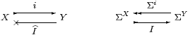
The effect of this is that X carries the subspace topology inherited from Y, in a canonical way: for an open subobject φ of X, it provides a particular open subobject Iφ of Y for which the restriction Σi(Iφ) is φ.
In the case where X is an open subobject of Y (Lemma 3.8), Iφ≡∃iφ is the least such extension, whilst for a closed subobject, Iφ≡∀iφ is the greatest one, but in general it need not be either of these.
The computational significance of Σ-split embeddings is that any observation (computation of type Σ) on the subobject extends canonically, though not uniquely, to the whole object.
Warning 7.2 Let Y⇉ Z be a parallel pair of continuous functions
between locally compact sober spaces
and X≡{y:Y ∣ f y=g y:Z} the subset of points that satisfy
the equation.
We give X the subspace topology,
i.e. its open subspaces are the restrictions of those of Y.
This is the equaliser X↣ Y⇉ Z
in the category of sober topological spaces,
but X need not be locally compact (or have an effective basis).
Equalisers also exist in the category of locales,
but again need not be locally compact, or even spatial.
Σ-split subspaces are therefore a very special case.
Remark 7.3 For this reason,
the formulation of ASD that we gave in Axiom 3.3(c)
does not provide general equalisers.
It formally adjoins
(Section B 4) a Σ-split subobject i:X≡{Y ∣ E}↣ Y of Y
with I:ΣX◁ΣY
such that Σi· I=idΣX and I·Σi=E,
given any endomorphism E:ΣY→ΣY
that satisfies the appropriate equation.
We shall consider the formulation of this equation
in Section 10.
The λ-calculus developed in
Section B 8 allows arbitrarily complicated combinations of Σ-split subobjects
and exponentials,
but in this section and the next we reduce them to
Σ-split subobjects of ΣN.
The following results link three (d–f) of the abstract characterisations of local compactness in the Introduction.
Lemma 7.4 Any object X that has an effective basis
(βn,An) indexed by N is a Σ-split subobject of
ΣN.
Proof Using the basis (βn,An), define
|
Then Σi(Iφ) = λ x.(Iφ)(i x) = λ x.∃ n. Anφ∧βn x = φ. We also recover
| x = focus(∃ n.An∧ξ n). ▫ |
Incidentally, notice the use of letters here: we write x:X, φ:ΣX and F:ΣΣX for the object under study, but n:N, ξ:ΣN and Φ:ΣΣN for its basis, the idea being that x and φ are represented by ξ and Φ under the embedding.
Conversely, any Σ-split subobject inherits the basis of the ambient object, using the inverse images of the basic open subobjects along i:X↣ Y. However, for the compact subobjects, we use their direct images along the “second class” map

in the sense of Remark 5.14. Since I need not preserve meets, nor need the modal operator ΣI A≡ A· I. This is why we find bases in which An need not preserve ⊤ and ∧.
Lemma 7.5 Let (βn,An) be an effective basis
for Y and i:X↣ Y a Σ-split subobject.
Then (Σiβn,ΣI An) is an effective basis for X.
If an ∨- or ∧-basis was given, the result is one too.
If An is a filter and I preserves ⊤ and ∧
then ΣI An is also a filter.
In other words, Σ-split subobjects of locally compact objects are again locally compact.
Proof For φ:ΣX, Iφ:ΣY has basis decomposition
| Iφ ⇔ ∃ n.An(Iφ)∧βn ≡ ∃ n.(ΣI An)φ∧βn. |
Since Σi is a homomorphism, it preserves scalars, ∧ and ∃, so
| φ = Σi(Iφ) = Σi(∃ n.An(Iφ)∧βn) = ∃ n.An(Iφ)∧Σiβn. ▫ |
Corollary 7.6 4.10) defined a basis on
ΣN. ▫
These two constructions are not inverse: given an N-indexed effective basis on X, we obtain a Σ-split embedding X↣ΣN, and then a basis indexed by Fin(N). In Lemma 15.6 we shall want to recover the original, N-indexed, basis.
Lemma 7.7
An embedding X↣ΣN arises from a basis
according to Lemma 7.4 iff each Iφ preserves joins.
It’s then a filter basis iff, for each n,
λφ.Iφ{n} also preserves finite meets.
Proof For any basis, ξ↦ Iφξ≡∃ n. Anφ∧ξ n preserves joins. Conversely, with
| βn ≡ λ x.i x n and An ≡ λφ.Iφ |
|
we recover φ x ≡ (Iφ)(i x) ⇔ ∃ n.Iφ{n}∧ i x n ⇔ ∃ n. Anφ∧βn x so long as Iφ preserves the join i x=∃ n.i x n∧{n}. ▫
In the rest of this section we consider the classical interpretations of the Σ-split embedding that arises from an effective basis, starting with traditional topology. Recall from [Joh82, Theorem II 1.2] that the free frame on N is ΥK N (the lattice of upper subsets of K N), and that this is isomorphic to the lattice of Scott-open subsets of the powerset ℘(N).
Theorem 7.8 Let X be a locally compact sober space with
N-indexed basis (Un,Kn). Then X is a Σ-split subspace
of ℘(N).
Proof The embedding in Lemma 7.4 takes
|
The second map, I, is Scott-continuous because it takes ⋃s↑ Vs to
| {ℓ ∣ ∃ n∈ℓ.Kn⊂⋃s↑ Vs} = {ℓ ∣ ∃ n∈ℓ.∃ s.Kn⊂ Vs} = ⋃s↑{ℓ ∣ ∃ n∈ℓ.Kn⊂ Vs}. |
The composite Σi· I takes V⊂ X to ⋃ {⋂n∈ℓUn ∣ ∃ n∈ℓ.Kn⊂ V}, and by Definition 1.1, this contains V={x ∣ ∃ n.x∈ Un⊂ Kn⊂ V}. For the converse, if x∈Σi(I V) then ∃ℓ.∀ n∈ℓ. x∈ Un∧ ∃ m∈ℓ.Kn⊂ V, so ∃ n.x∈ Un⊂ Kn⊂ V. ▫
Example 7.9 A compact Hausdorff space has a basis determined by a family
of disjoint pairs (Un⋔ Vn) of open subspaces.
In this case, the embedding is
|
Consider in particular the embedding of ℝ in ΣN, where N indexes a basis of open and closed intervals (Examples 1.4 and 6.10). This is closely related to one of the first examples that Dana Scott used to show how continuous lattices could be used as a model of computation [Sco70].
Definition 7.10
The lattice of intervals, Iℝ⊤,
of ℝ is the set of convex closed subspaces
(including the empty one),
ordered by reverse inclusion, and given the Scott topology.
The domain of intervals, Iℝ⊂Iℝ⊤,
consists of the inhabited such subspaces.
Amongst these, points of ℝ are identified with
the maximal elements.
Classically, the members of Iℝ are of the form
[r±δ], with r∈ℝ and 0≤δ≤∞.
Remark 7.11 In ASD, closed subobjects under reverse inclusion
correspond to their co-classifiers under the (forward) intrinsic order,
and to the “complementary” open subobjects under inclusion.
When the closed subobject is convex, the open one is δ∨υ,
where δ is lower and υ upper in the arithmetical order,
so the pair (δ,υ) is almost a Dedekind cut [I],
except that it is disjoint but need not be “located”.
It has this last property exactly when the closed subobject is a singleton.
Intervals [p,q] or [r±δ] with specified endpoints are of this form, but (in ASD and other constructive forms of analysis), not every inhabited convex closed bounded subobject need have endpoints. It does so iff it is also overt [J]. In particular, a directed join in Iℝ of subobjects with endpoints need not itself have them.
It is, however, not necessary to appreciate this issue in order to see the relationship between Iℝ and our representation of ℝ as a Σ-split subobject of ΣN.

where N is the set of pairs, written <q±є>, with є>0 and q rational.
(Recall that the square tail indicates a closed inclusion.)
Proof The embedding takes r∈ℝ to [r±0] and then to λ<q±є>.r∈(q±є), which is (the exponential transpose of) a continuous function. The retraction is defined by intersection:
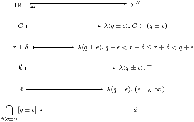
Any compact interval of the T1 space ℝ is saturated in the sense of Lemma 5.15. It is therefore the intersection of its open neighbourhoods, amongst which open intervals suffice. Hence the composite is Iℝ⊤→ΣN→Iℝ⊤ is the identity.
The projection Iℝ⊤↞ΣN is Scott-continuous because it clearly takes directed unions of sets of codes to codirected intersections of compact subspaces. Classically, Lemma 5.17 showed that such intersections correspond to unions of neighbourhood filters, whilst in ASD they correspond to the unions of the complementary open subobjects δ∨υ. Hence the inclusion Iℝ⊤↣ΣN is also Scott-continuous.
The inverse image of ⊤ under Iℝ⊤↞ΣN is the open subobject classified by the inconsistency predicate
| InCon(φ) ≡ ∃<q1±є1><q2±є2>. (q1+є1< q2−є2) ∧φ<q1±є1>∧φ<q2±є2>. |
The complementary closed subobject of ΣN is of course not classified, as it’s not open, but when we restrict attention to its (overt discrete collection of) finite elements, we find that consistency is characterised by the decidable formula
| Con(ℓ) ≡ ∃ x:ℚ.∀<q±є>∈ℓ.x∈<q±є>, |
so
| InCon(λ<q±є>.<q±є>∈ℓ) = ¬Con(ℓ). ▫ |
Remark 7.13
The idea behind the domain of intervals is not hard to generalise.
Indeed, we may embed any locally compact sober space as a subspace of
its continuous preframe of compact saturated subspaces (Theorem 5.18),
each point being represented by its saturation in
the sense of Lemma 5.15.
That the image consists of the maximal points (excluding ∅)
plainly depends on starting with a T1-space,
so can’t be an essential feature of the construction.
Another interesting aspect of the general construction is the decidable consistency predicate on finite elements. Scott developed these into what became a standard form of domain theory [Sco82]. The subobject of ΣN that is determined by the consistent elements is closed, but also overt [F].
We shall develop our own construction of the real line via Dedekind cuts, and also discuss the interval domain further, in [I].
Now we give the localic version of Theorem 7.8. This result is the most efficient way of establishing the connection between locally compact locales and ASD.
Theorem 7.14
Let L be any N-based continuous distributive lattice.
Then there is a frame homomorphism H and a Scott-continuous function I
with H· I=idL, as shown:
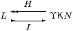
Conversely, any lattice L that admits such a pair of functions is continuous and distributive.
Proof [⇒] Let (βn) be a basis for the continuous lattice L and An≡λφ.(βn≪φ). Let H:ΥK N→ L be the unique frame homomorphism that extends β(−):N→ L, so
| for U∈ΥK N, HU = ⋁ℓ∈U⋀n∈ℓβn ∈ L, |
and define I:L→ΥK N by Iφ = {ℓ ∣ ∃ n∈ℓ.βn≪φ}. This is Scott-continuous by a similar argument to that in Theorem 7.8, with βn≺≺φs instead of Kn⊂ Vs. Then
|
from which we deduce H(Iφ)=φ, because (βn) is a basis.
[⇐] Conversely, if such a diagram exists then I· H is a Scott-continuous idempotent on a continuous lattice, so its splitting L is also continuous [Joh82, Lemma VII 2.3]. As H preserves joins, it has a right adjoint, H⊣ R, so id≤ R· H≡ j=j· j, and R preserves meets but not necessarily directed joins. Since H also preserves finite meets, so does j, and this is a nucleus in the sense of locale theory [Joh82, Section II 2.2], so its splitting L is a frame. ▫
Any locally compact locale is therefore determined by a Scott-continuous idempotent E on ΥK N. It is not just an idempotent, however, since the surjective part of its splitting must be a frame homomorphism. Since the latter preserves ⊤ and ⊥ by monotonicity, and ⋁↑ as E is Scott-continuous, it is enough to identify the condition on E the ensures preservation of the two binary lattice connectives, which we may treat exactly alike. (This is where Remark 3.4 came from.)
Lemma 7.15 Let I and H be monotone functions between two
semilattices, with H· I=id. Then H preserves ∧ iff
E≡ I· H satisfies the equation E(φ∧ψ) =
E(Eφ∧ Eψ).
Proof If H preserves ∧ then
|
For the converse, note first that we have H(φ∧ψ)≤ Hφ∧ Hψ and I(φ′∧ψ′)≤ Iφ′∧ Iψ′ by the definition of ∧. Then
|
so H(φ∧ψ)≤ Hφ∧ Hψ≤ H(φ∧ψ). ▫
Corollary 7.16 Any N-based locally compact locale is determined by
a Scott-continuous endofunction of the frame ΥK N
(or by a locale endomorphism of ΣΣN) such that
| E(φ∧ψ) = E(Eφ∧ Eψ) and E(φ∨ψ) = E(Eφ∨ Eψ). ▫ |
We now have to concentrate on the logical development within abstract Stone duality, and will only return to the connection with traditional topology in Section 17. The first task is to show that every definable object has an effective basis, and is therefore a Σ-split subobject of ΣN. Such subobjects are determined by idempotents E on ΣΣN satisfying the equation that we have just identified, along with its counterpart for ∨. However, even that characterisation depends on the use of bases (Lemma 10.7ff).