


We now return to Richard Dedekind’s construction of the real line, which we introduced in Section 2. Whilst this is very familiar, we need to be sure that it can be carried out in our very weak logic. We begin with what we require of the rationals for the purposes of topology, postponing arithmetic to Sections 11–13. Both the ingredients (Q) and the result (R) of the construction satisfy the first definition, but we shall use combinatorial operations on the rationals which will rely on decidable equality (Remark 6.15).
Definition 6.1 A dense linear order without endpoints
is an overt Hausdorff object Q (Definitions 4.12 and 4.14)
with an open binary relation < that is, for p,q,r:Q,
|
The ∃ q in the interpolation axiom does not necessarily mean the midpoint ½(p+r). It might instead mean the “simplest” interpolant, in some sense, as in John Conway’s number system [Con76]. In practical computation, the best choice of q may be determined by considerations elsewhere in the problem, cf. unification in Prolog (Remark 3.4).
|
Lemma 6.3 If Q is discrete then = and < are decidable,
with (p≮ q)≡(p=q)∨(q< p).
This is the case when Q is countable
(by which we mean strictly that Q≅ℕ, Remark 5.22),
in which case the usual order on ℕ induces
another (well founded) order ≺ on Q that we call simplicity.
▫
Examples 6.4 Such countable Q may consist of
where in all cases < is the arithmetical order. For the sake of motivation and of having a name for them, we shall refer to the elements of any such countable Q as rationals, but for a particular target computation any of the above structures may be chosen. We keep the dyadic rationals in mind for practical reasons, but they have no preferred role in the definition.
Proposition 6.5 Any two countable dense linear orders without endpoints are order-isomorphic.
Proof The isomorphism Q1≅ Q2 is built up from finite lists of pairs (Theorem 5.21) by course-of-values recursion and definition by description (Axiom 4.24). Given such a list, we may add another pair that consists of the simplest absentee from Q1, together with its simplest order-match from Q2. At the next stage, we start with an absentee from Q2. ▫
Remark 6.6 Of course, this well known model-theoretic result misses the
point of real analysis.
When we apply it to different notions of “rationals”,
it destroys the arithmetic operations and the Archimedean property
(Axiom 11.2).
In Definition 13.1 we shall show how order automorphisms
(strictly monotone functions) of R arise from relations
rather than functions on Q.
Remark 6.7 There are many formulations of Dedekind cuts.
We choose a two-sided version that appears as Exercise 5.3.3 in
[TvD88],
but we don’t know who originally formulated it.
That book, like many other accounts, uses a one-sided version
in its main development.
As in the case of open and closed subspaces (Remark 3.2f), the relationship between the two sides of the cut is contravariant. One-sided accounts obtain one from the other by means of (Heyting) negation — with some awkwardness, since arithmetic negation ought to be involutive, whereas logical negation is not, in intuitionistic logic.
The ASD calculus does not allow negation of predicates. Nor, indeed, is there any kind of contravariant operation, as it would be neither continuous nor computable. So we have to use both halves of the cut. But this is not just to overcome a technical handicap of our weak logic: like open and closed subspaces, the two parts play complementary roles that are plainly of equal importance. We also saw in Section 2 that it is natural to generalise Dedekind cuts by not forcing the halves to be complementary, the resulting space being the interval domain.
Definition 6.8
Formalising Remark 2.1,
a (Dedekind) cut (δ,υ)
in a (not necessarily discrete) dense linear order without endpoints
(Q,<) is a pair of predicates
| for d,u:Q, δ d, υ u:Σ, |
possibly involving parameters, such that
|
We call δ or υ rounded if they satisfy the first or second of the above properties, these being the most important. Their types are the ascending and descending reals (R, R, Example 2.8 and Definition 7.3). Lemma 7.5 explains why we have defined disjointness in this way, in preference to several others, and we shall discuss a stronger notion of locatedness that is needed for arithmetic in Proposition 11.15. When (δ,υ) are rounded, bounded and disjoint, they represent an interval (Definitions 2.3 and 7.8). We construct the space IR of intervals in the next section, on the way to the construction of R itself.
We do not introduce the “set” of cuts. However, we reformulate this definition using a little category theory to provide the context in which to understand both our construction in ASD and the alternatives in other foundational settings in Section 15.
Remark 6.9 The six axioms above
are (essentially) equations (cf. Axiom 4.5).
The boundedness axioms are already equations between terms of type Σ,
whilst the roundedness and disjointness conditions become equations of type
ΣQ and ΣQ× Q when we λ-abstract the variables.
Finally, locatedness may be rewritten as
| (λ d u.δ d∨υ u∨(d< u)) = (λ d u.δ d∨υ u) of type ΣQ× Q. |
We therefore expect R to be the subspace of ΣQ × ΣQ of those pairs (δ,υ) that satisfy these six equations. In the language of category theory, this is the equaliser (Definition 5.3) of the parallel pair of arrows that collects them together:
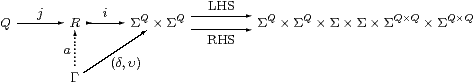
We shall explain how to construct this equaliser in ASD, i.e. to define the new type R of Dedekind cuts, in the next two sections. For the remainder of this one, Definition 6.8 is merely a list of properties that a pair of predicates on Q may or may not have.
Real numbers admit two order relations, which we shall now define in terms of cuts. Recall from Remark 4.6(b) that we expect a< b to be a predicate (a term of type Σ) but a≤ b to be a statement (an equation between such terms).
Definition 6.10
The irreflexive (strict) order relation on cuts is the predicate
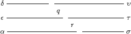
| (δ,υ)<(є,τ) ≡ ∃ q.υ q∧ є q. |
The idea is that the right part of the smaller cut overlaps the left part of the larger.
Lemma 6.11 The relation < is transitive.
Proof
Lemma 6.12
As in Remark 2.1,
each q:Q gives rise to a cut j q≡(δq,υq) with
| δq ≡ λ d.(d< q) and υq ≡ λ u.(q< u). |
Beware that q is a sub-script! This is an order embedding, in the sense that
| (q< s) ⇔ (∃ r.q< r< s) ⇔ (∃ r.υq r∧δs r) ≡ ((δq,υq)<(δs,υs)). |
The map j makes Q an example of the test object Γ in the equaliser diagram above. Then the map Q→ΣQ×ΣQ by q↦(δq,υq) is mono (1–1), as is j:Q→ R. ▫
When we compare a real number (i.e. a cut) with a rational, we recover the lower or upper part of the cut:
Lemma 6.13 (δd,υd)<(δ,υ) ⇔ δ d and (δ,υ)<(δu,υu) ⇔ υ u. ▫
We would like to show next that < is interpolative and extrapolative, but even to say that we need ∃R, for which we have to define R itself as a type in ASD, so we leave this until Section 9.
Now we consider the reflexive (non-strict) order ≤. This is given by implication or inclusion between the cuts considered as predicates or subsets.
Proposition 6.14
Let (δ,υ) and (є,τ) be cuts,
possibly involving parameters. Then the three statements
| δ⊒є:ΣQ, υ⊑τ:ΣQ and ((δ,υ)<(є,τ)) ⇔ ⊥ |
are equivalent. We write (є,τ)≤(δ,υ) for any of them. Notice that the arithmetical order ≤ agrees with the logical one ⊑ for the ascending reals δ and є, but is the reverse for the descending reals τ and υ, cf. Example 2.8.
Proof Since ((δ,υ)<(є,τ)) is ∃ q.υ q∧є q, it is ⊥ if either є⊑δ or υ⊑τ, since cuts are rounded and disjoint.
Conversely, by the definition of ∃, another way of writing the statement with < is
| for any q:Q, (υ q∧є q) ⇒ ⊥ |
Then, for p:Q,
|
and similarly υ p⇒τ p. ▫
There is one more order-theoretic property that we shall need: it develops the notion of order-locatedness a little towards arithmetic, for which the stronger definition will be needed. The fact that this Lemma does not require disjointness, and so also applies to the back-to-front intervals in Remark 2.20, will become relevant when we study the existential quantifier.
Remark 6.15 We present this proof in the usual informal style,
in which “⋯” indicates the variable length of the list,
but the formal proof, of course, uses list induction.
In particular, the ordering of the list is an open predicate that,
like the n-fold conjunction, is easily definable by recursion on lists.
This means that we rely on the methods of “discrete mathematics”
that were outlined in and following Theorem 5.21,
but these only work for overt discrete spaces.
On the other hand, for Definition 6.1 it had to be Hausdorff,
so equality on Q must be decidable,
cf. Lemmas 4.13 and 6.3.
Lemma 6.16 Let q0< q1<⋯< qn
be a strictly ascending finite sequence of rationals,
and let (δ,υ) be rounded, located and bounded,
with δ q0 and υ qn.
Then this (pseudo-)cut belongs to at least one of the overlapping
open intervals
| (q0,q2), (q1,q3), …, (qn−2,qn), |
in the sense that
| ⋁j=0n−2(δ qj∧υ qj+2). |
Proof The hypotheses δ q0 and υ qn and order-locatedness of (δ,υ) applied to each pair qj< qj+1 give
| δ q0 ∧ (δ q0∨υ q1) ∧ (δ q1∨υ q2) ∧ ⋯ ∧ (δ qn−1∨υ qn) ∧ υ qn, |
which we expand using distributivity. Of the 2n disjuncts, n+1 yield those in the claim, including two repetitions:
|
Each of the remaining 2n−n−1 disjuncts consists of a conjunction of δs up to some δ qj and of υs starting from υ qi, with 1≤ i≤ j+1≤ n. Such a conjunction vanishes if δ and υ are disjoint. But even if they are not, since υ is upper we have
| δ qj∧ υ qi =⇒ δ qj∧υ qj+2, |
which is one of the disjuncts in the claim. ▫
Exercise 6.17 Formulate the following in accordance with
Remark 4.6, and prove them:
Finally, verify that the results about < and ≤ make no use of the boundedness axiom for cuts, and therefore also apply to +∞≡(⊤,⊥) and −∞≡(⊥,⊤). ▫