


In this section we prove that the closed interval is compact and overt, in the sense of Definition 4.14, namely that it admits both “quantifiers”, ∀ and ∃. The constructions formalise in ASD some of the ideas that we met in the context of interval analysis in Section 2. We compute the universal quantifier ∀ x:[d,u].φ x by splitting the interval into sufficiently but finitely many sub-intervals, and applying φ to each of them à la Moore. The existential quantifier, on the other hand, is related to the back-to-front (Kaucher) intervals that we saw in Remark 2.20.
First, of course, we have to construct the closed interval itself, and for the sake of symmetry the open one too, as objects of ASD. These are defined by means of terms of type ΣR.
Definition 10.1
For d≤ u:R, the open and closed intervals
(d,u),[d,u]⊂ R are
More generally, for any rounded pair (δ,υ),
where we expect the pseudo-cut (δ,υ) to be located (maybe overlapping or back-to-front) in the first case and disjoint in the second.
Remark 10.2
The ASD subspaces that are defined by these terms were constructed in
Remarks 5.8ff.
However, as we have not allowed dependent types in the calculus,
we must temporarily restrict attention to intervals with constant endpoints,
so d, u, δ and υ cannot have parameters.
In other words, we are essentially just dealing with the unit interval
I≡[0,1], where d≡0, u≡1.
But this is no real handicap, since (when we have some arithmetic)
the general interval [d,u] with endpoints
will be the direct image of [0,1] under the function t↦ d(1−t)+u t
(Proposition J 9.6).
This actually generalises to all rounded bounded (δ,υ)
(Lemma J 9.10).
The outcome is that the formulae that we obtain in the end
remain valid with parametric endpoints.
Even if we had a theory of dependent types and tried to use it to prove the results in this section, we would still have to demonstrate that the formulae that look like nuclei or quantifiers actually correspond to (dependent) subspaces. That would be at least as difficult as the approach that we take here.
On the other hand, terms with parameters have been familiar for centuries, and translate more directly into programs. In Section J 14 we will use modal operators (quantifiers over subspaces) derived from f as a tool for solving the equation f(x)=0, naturally involving the same parameters as the function. These operators are (Scott) continuous in the parameters, which means that we may still work with them in the vicinity of singularities of the equation, where the sets or types of zeroes are discontinuous.
Proposition 10.3
Any open subspace U⊂ R classified by θ:ΣR is overt.
This applies in particular to the open intervals (d,u) and
(υ,δ) in Definition 10.1.
The existential quantifiers are defined for φ:ΣR by
|
in which ∃ x:R was defined in Theorem 9.2 and is the same as ∃ x:Q.
Proof We may deduce in both directions:
|
so ∃ x:R.θ x∧φ x satisfies the defining property of ∃ x:U.φ x. ▫
Remark 10.4 The main task of this section is to show that, for d≤ u,
the closed interval [d,u] is overt and compact.
The quantifiers ∃ and ∀ will be given by
| ∃ x:[d,u].φ x ⇔ E1Φ(δu,υd) ⇔ EΦ(δu,υd) and ∀ x:[d,u].φ x ⇔ EΦ(δd,υu), |
where Lemma 8.10 allows us to interchange E with E1 in the existential quantifier, because the argument (δu,υd) is located.
Here Φ:ΣQ×ΣQ→Σ is any extension of φ:R→Σ. As in Remark 2.5, the canonical one is Φ≡ Iφ, but the Moore–Kaucher interpretation of the arithmetical operations may be used to find another extension in a more practical way. In any case, the notation is simpler if we put things the other way round, working primarily with Φ, so that φ x≡Φ(i x)≡Φ(δx,υx).
We first show that the closed interval, like the open one, is overt, by a generalisation of Theorem 9.2. Since E1 preserves ⊥, this may also be seen as an application of Lemma 5.13 to the lattice R×R↓(δu,υd) of rounded pseudo-cuts with (δ,υ)≤(δu,υd). Recall that L↓α means {β:L ∣ β⊑α}.
Proposition 10.5
The closed interval [d,u] is overt, with
∃ x:[d,u].Φ(i x) ≡
E1Φ(δu,
υd).
|
Notice that, as in Remark 2.20, u and d are the “wrong” way round.
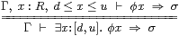
Proof This is similar to Proposition 10.3. By Lemma 9.1, the top line of the rule is
| Γ, x,d,u:R, d≤ x≤ u ⊢ φ x ≡ ∃ e t.e< x< t∧Φ(δe,υt) ⇒ σ, |
which, by Definition 4.14 (for ∃) and Axiom 4.7, is equivalent to
| Γ, x,d,u,e,t:R, d≤ x≤ u, e< x< t ⊢ Φ(δe,υt) ⇒ σ. |
The inequalities on the left of the ⊢ are equivalent to
| d≤ u, max(d,e) ≤ x ≤ min(t,u), e< t, e< u, d< t, |
the last three of which can be moved back across the ⊢, using Definition 4.14 and Axiom 4.7 again, whilst x is now redundant. Hence
| Γ, d,u:R, d≤ u ⊢ E1Φ(δu,υd) ≡ ∃ e< t.e< u∧ d< t∧Φ(δe,υt) ⇒ σ, |
which is the bottom line of the rule. ▫
Exercise 10.6 Show that
∃ x:[d,u].φ x =⇒
φ d∨(∃ x:R.d< x< u∧φ x)∨ φ u. ▫
Now we come to the principal result of this paper, that the closed interval [d,u] is compact. The proof may be considered as another example of Lemma 5.13, with
| [d,u] ⊂ {(δ,υ):IR ∣ δd⊑δ & υu⊑υ}. |
Theorem 10.7 The closed interval [d,u]⊂ R
is compact in the sense of Definition 4.14:
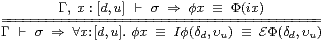
|
Proof In the upward direction, let (δ,υ)≡(δx,υx)⊒(δd,υu) be the cut corresponding to x:R. Then
| Γ ⊢ σ ⇒ Iφ(δd,υu) ⇒ Iφ(δ,υ) ≡ Iφ(i x) ⇔ φ x. |
For the converse, first let ψ ≡ λ x.(x> u∨ x< d):ΣR and Ψ≡λαβ.α u∨β d:ΣΣQ×ΣQ, so ψ=ΣiΨ co-classifies [d,u] (Definition 10.1). Using Axiom 4.7, the top line says
| Γ, x:R ⊢ φ x∨ψ x ≡ φ x∨(x< d)∨(x> u) ⇔ ⊤. |
This captures universal quantification as a judgement (Definition 4.4). By λ-abstraction,
| Γ ⊢ Σi(Φ∨Ψ) = ΣiΦ∨ΣiΨ = φ∨ψ = ⊤ = Σi⊤:ΣR, |
so if we apply I to this, where E=I·Σi, and the result to (δd,υu), we have
| E(Φ∨ Ψ)(δd,υu) ⇔ E⊤(δd,υu) ⇔ ⊤ |
by Lemma 8.5. In the expansion of E(Φ∨ Ψ)(δd,υu), the same Lemma uses conjuncts like
| (Φ∨ Ψ) (δqk,υqk+1) ⇔ Φ(δqk,υqk+1) ∨ (u< qk ∨ qk+1< d) ⇔ Φ(δqk,υqk+1) ∨ ⊥. |
Hence
| ⊤ ⇔ E Φ(δd,υu) ⇔ E(Φ∨ Ψ)(δd,υu). ▫ |
Corollary 10.8
Re-substituting Definition 8.2 of E,
|
using Notation 7.1, Lemmas 8.3, 8.5 and 9.1 and Proposition 10.5. ▫
Warning 10.9
In view of the fact that both quantifiers are given by almost the same
formula, the hypothesis d≤ u must be important.
If we do not know this, we can still obtain the bounded universal
quantifier as
| (∀ d≤ x≤ u.Φ(i x)) ≡ (d> u) ∨ EΦ(δd,υu), |
but for the existential quantifier we have to write
| Φ:ΣΣQ×ΣQ, d≤ u:R ⊢ ∃ d≤ x≤ u.Φ(i x) ≡ EΦ(δu,υd). |
This is because (∃ d≤ x≤ u.⊤)⇔ ⊤ ⊣⊢ (d≤ u) ⊣⊢ (d> u)⇔ ⊥, making a positive statement equivalent to a negative one. But that would make the predicate (d> u) decidable, which it can only be if we had already assumed that it was either true or (in fact) false.
Notice that the intersection of two overt subspaces need not be overt, even in the simple case of [d,u]∩[e,t]. This is because we need to be able to decide whether they are disjoint (t< d∨ u< e) or overlap (t≥ d & u≥ e). We shall see more examples of this in Section J 16.
While we’re looking at awkward cases, recall from Theorem 9.2 that
| ∃ x:R.Φ(i x) ⇔ EΦ(⊤,⊤), |
and it’s easy to check that ∃ x≤ u.Φ(i x) ⇔ EΦ(δu,⊤) and ∃ x≥ d.Φ(i x) ⇔ EΦ(⊤,υd) .
So what happens if we let one or both of the arguments of EΦ be ⊥? Does this give a meaning to φ(∞)≡limx→∞φ x or to ∀−∞≤ x≤∞.φ x? Unfortunately not: putting δ or υ≡⊥ in Notation 8.2 just gives ⊥. ▫
Remark 10.10
You are probably wondering where the “finite open sub-cover” has gone.
Essentially, it was absorbed into the axioms, in the form of general
Scott continuity (Axiom 4.21).
Compactness is often said to be a generalisation of finiteness. We dissent from this. The finiteness is a side-effect of Scott continuity. The essence of compactness lies, not in that the cover be finite, but in what it says about the notion of covering. Recall how the statement of equality became an (in)equality predicate in a discrete or Hausdorff space (Remark 4.6). Similarly, compactness promotes the judgement (Definition 4.4),
| …, x:[d,u] ⊢ φ x⇔⊤, |
that an open subspace covers into a predicate (Axiom 4.2),
| ∀ x:[d,u].φ x ≡ Iφ(δd,υu) ⇔ ⊤. |
Now, λφ.∀ x:[d,u].φ x is a term in the ASD λ-calculus of type ΣΣR, and, like all such terms, it preserves directed joins. So if φℓx is directed with respect to ℓ:D then
| ∀ x:[d,u]. ⋁ℓ↑ φℓx ⇔ ⋁ℓ↑∀ x:[d,u].φℓx. |
Restating this for general joins, we have
| ∀ x:[d,u]. ∃ n:N. φn x ⇔ ∃ℓ:Fin(N). ∀ x:[d,u].∃ n∈ℓ.φn x, |
where ℓ provides the finite open sub-cover.
Now, it is a little surprising that the Heine–Borel property is traditionally expressed using finite open sub-covers, when a very common situation in analysis is that the cover is indexed by the real numbers, which are directed. In this case, just one member of the family covers, and we have uniform values, for example
| ∀ x:[d,u].∃δ> 0.φδx ⇔ ∃δ> 0.∀ x:[d,u].φδx, |
so long as φ is contravariant in the sense that δ≤є ⊢ φє ⇒ φδ. ▫
Warning 10.11
Our “∃ℓ:Fin(N)” and ∃δ> 0
do not have the same strength as they do in other constructive systems.
The computational implementation only produces ℓ or δ
in the case where the predicate (is provably true and) has at worst
variables of type ℕ (Remark 3.5).
In particular, if the predicate φ (and maybe even the bounds d and u)
are expressions with real-valued parameters,
neither δ nor even the length of the list ℓ
can be extracted as functions of these parameters.
Lemma 10.12 The open interval (0,1) is not compact.
Proof By Definition 6.10 for 0< x,
| x:(0,1) ⊢ ⊤ ⇔ ∃ q:Q.0< q< x, |
where ∃ is directed, so if (0,1) were compact we could interchange the quantifiers, but
| ⊤ ⇔ ∀ x:(0,1).∃ q> 0.q< x ⇔ ∃ q> 0.∀ x:(0,1).q< x ⇔ ⊥. ▫ |