


Now we can begin to develop some general topology and logic in terms of the Euclidean and Phoa principles and monadicity.
For the remainder of the paper (apart from the last section), we shall work in a model (C,Σ) of the axioms in Remark 3.8, i.e. Σ is a Euclidean semilattice and the adjunction is monadic. The category could be Set, LKLoc, CDLatop, an elementary topos or a free category as considered in Theorem 4.2 and Remark 4.3. We shall also assume the dual Euclidean principle when discussing the dual concepts: closed subspaces, compact Hausdorff spaces and proper maps.
By Theorem 3.10, Σ classifies some class M of supports, which we call open inclusions. So far, M has been entirely abstract: the only maps that are obliged to belong to it are the isomorphisms. The diagonal map Δ:X→ X× X is always a split mono, so what happens if this is open or closed?
In accordance with our convention about Greek and italic letters (Remark 2.5), we use p0:X× Y→ X and p1:X× Y→ Y instead of the more usual π for product projections, though we keep Δ for the diagonal.
Definition 6.1 An object X∈obC is said to be
discrete if the diagonal X↪ X× X is open.
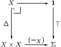
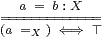
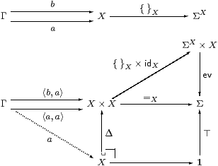
The characteristic map (=X):X× X→Σ and its transpose { }X:X→ΣX are known as the equality predicate and singleton map respectively. We shall often write the subscript on this extensional (but internal) notion of equality, to distinguish it from the intensional (but external) equality of morphisms in the category C.
[Symbolically, the equality predicate =X is related to equality of morphisms by the rule
|
in which a=b:X is called a statement in Definition I 4.4.]
Lemma 6.2
If X is discrete in this sense then it is T1,
i.e. the Σ-order (Definition 1) on X is discrete.
If all functions Σ→Σ are monotone
then the link order is also discrete.
Proof If x⊑Σy then {x}⊑Σ{y} in ΣX by Remark 5.10(a), so, by putting φ≡evx in the definition of ⊑Σ, by reflexivity we have ⊤⇔ {x}(x)⊑{y}(x)≡(x=X y).
If all F:Σ→Σ are monotone then x⊑L y⊢ x⊑Σy. But for a direct argument (on the same hypothesis) consider F≡λσ.(ℓσ=Xℓ⊥). Then F⊥⇔ ⊤, so F⊤⇔ ⊤ by monotonicity, but this says that x=X y. ▫
Definition 6.4
Dually, we say that an object is Hausdorff if the diagonal is closed
(classified by ⊥) [Bou66, §8].
We write (≠X) or (#X):X× X→Σ
for the characteristic function,
which is sometimes called apartness.
Again, it follows that singletons are closed
(the T1 separation property in point-set topology),
but not arbitrary subsets.
The symbolic rule is
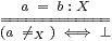
|
Exercise 6.5
To check that you understand how ≠X is defined,
adapt Lemma 6.2 to show that
if x⊑Σy in a Hausdorff space X then (x≠X y)⇔ ⊥,
and explain how it follows from this that X is T1
in the order-theoretic sense. ▫
To sum up, discreteness and Hausdorffness are quite different properties.
Lemma 6.7
Let X be discrete and φ∈ΣX. Then
| ∃Δ(φ) ≡ (λ x y.(x=X y)∧ φ x) ≡ (λ x y.(x=X y)∧ φ y). |
Proof We use the Frobenius law ∃Δ(θ∧ΣΔψ)≡ (∃Δθ)∧ψ, with θ≡⊤, so (∃Δθ)=(λ x y.x=X y). Putting either ψ≡Σp0φ or Σp1φ, so ψ=λ x y.φ(x) or λ x y.φ(y), we recover φ=ΣΔψ, so the left hand side of the Frobenius law is ∃Δ(φ) and the right hand side is one of the other two expressions.
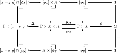
Theorem 3.10 gives an alternative proof using open subsets: [(x=X y)∧ φ x] is the same subobject of Γ× X as [(x=X y)∧ φ y] since the composites X→ X× X⇉ X are equal; hence they are the also same subobject of Γ× X× X, so the characteristic maps are equal. ▫
Corollary 6.8 (=X) is reflexive, symmetric and transitive.
Proof Consider φ≡λ u.(y=X u) and φ≡λ u.(u=X z). ▫
This is the algebraic characterisation of the equality predicate, which we consider in Section 10.
Corollary 6.9 (λ n.φ(n)) a ≡ ∃ n.(n=ℕa)∧φ(n).
Here “∃ n” is as in Definition 7.7. So, instead of β-reducing the application of a predicate to an argument of type ℕ, i.e. substituting the term a for the variable n throughout the formula φ, we can make a local change to the expression-tree and rely on unification to carry out the effect of the substitution [Section A 11]. ▫
[Lemma J 5.9 proves the properties of equality symbolically from the Euclidean principle.]
Remark 6.10 The analogous property for ∀ in intuitionistic logic is that
| ∀Δ(φ)(x,y) ≡ (x=X y)⇒ φ x ≡ (x=X y)⇒ φ y. |
We need the dual Euclidean and Frobenius principles (Corollary 5.6) to make this equivalent to the lattice dual of the Lemma, namely
| ∀Δ(φ)(x,y) ≡ (x≠X y ∨ φ x) ≡ (x≠X y∨ φ y), |
for Hausdorff spaces. In this case, an object that is both discrete and Hausdorff is called decidable, cf. Proposition 9.6.
Proof [a,b] (=1)≡⊤:1×1→Σ
and (≠1)≡⊥.
[c,d] (=X× Y)≡(=X)∧(=Y)
and (≠X× Y)≡(≠X)∨(≠Y).
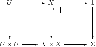
[e] U→ X is mono iff the square on the left is a pullback. ▫
The next result will be used to prove Theorem 11.3, so instead of monadicity we assume only that Σ is exponentiating, but still read the existence of the pullback in Definition 6.1 as the definition of discreteness.
Lemma 6.12
If X is discrete then the maps
{ }X:X→ΣX and ηX:X→ΣΣX are mono.
Proof If { }X∘ a={ }X∘ b then the composites Γ→Σ are equal, but one of them factors through the pullback, so the other does too.
Naturality of η with respect to { }X gives a commutative square
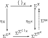
The map on the right is split mono, so by the first part and cancellation, ηX is mono. ▫
Remark 6.13 The Lemma helps to explain why
there are two ways of defining j-separated presheaves
(namely being T0 or discrete with respect to Ωj)
and the fact that Hausdorffness implies sobriety for spaces
[Joh82, Lemma II 1.6(ii)].
See also [Joh77, Definition 1.24],
[BW85, §2.3, Proposition 6]
and [Mik76, p. 3]
concerning the singleton map { }X in an elementary topos.
We shall find at the end of the paper that CDLatop satisfies most of our characterisation of elementary toposes, apart from the fact that all sets are discrete. Let’s briefly explore this analogy.
Example 6.14
Assuming excluded middle, the subcategory Set⊂Pos⊂CDLatop
consists of the discrete (equivalently, Hausdorff) objects.
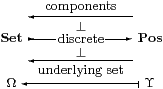
Set is the reflective subcategory of the Ω-replete objects in Pos, just as the sheaf subtopos ℰj consists of the Ωj-replete objects in ℰ [BR98].
The object Ω (the dominance in Set) is the underlying set of Υ (that in Pos), i.e. its image under the right adjoint of the inclusion Set⊂Pos. The product-preserving left adjoint (components) to the inclusion of categories is the replete reflection.
By contrast, Ωj is the result of applying the left adjoint, sheafification, to Ω. Also, we have Ω↞Υ instead of Ωj⊂Ω. ▫
Remarks 6.15
In the same way we may ask whether adjoints exist to the inclusions of
the full subcategories Set and KHaus
of (overt) discrete and compact Hausdorff spaces in LKLoc instead of Pos.
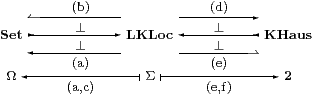
The lack of open–closed symmetry between these results makes it very unlikely that they have a unifying formulation in our axiomatisation.
[The overt discrete objects play the role of sets in ASD. If we assume, motivated by (a) above, that the inclusion of the full subcategory of them has a right adjoint U, then this subcategory is a topos with Ω≡UΣ and the whole category is equivalent to that of locally compact locales over this topos, [H].]
Discreteness and Hausdorffness are binary properties, relating X to X× X: we now turn to the corresponding nullary ones, involving 1=X0.