


In our new calculus, we will be able to reason about continuous, computable functions in ways that are quite similar to those with which you are already familiar for giving proofs based on set theory. So the situation is like that of learning Italian when your native language is Spanish: it’s possible to communicate quite effectively, but in order to learn the new language properly, you have to begin by defining the grammar of your own language in a more formal way. You may perhaps wish to hear the language being spoken (in the course of this paper) before learning it yourself, but this section is by no means optional.
Remark 5.1
Hermann Weyl (quoted in [EJ92])
said that “logic is the hygiene the mathematician
practices to keep his ideas healthy and strong”.
This precisely sums up what ASD provides,
if we take “health and strength” to mean that
any function that we define will be continuous automatically,
according to the right topologies on the object concerned.
We achieve this by enforcing “hygiene” precautions that take the form of restrictions on the applicability of the usual logical connectives. In other words, to gain the benefit of our calculus you need to learn the rules according to which these may be used in topology, and unlearn those that come from mathematics based on set theory, which yield non-continuous functions. As we shall see, these restrictions are topologically natural, for example the universal quantifier, ∀, may only range over compact spaces (Sections 2 and 8).
Our approach is in contrast to the traditional one that begins by allowing set-theoretic reasoning in its widest generality, and afterwards tries to restore sanity by imposing topological and computational structure. Our thesis is that this unwieldy structure is unnecessary, because the same things can be achieved more naturally by introducing a weaker logic that is in tune with topology and computation in the first place.
The style in which we shall set out our predicate calculus belongs to a tradition begun by Gerhard Gentzen [Gen35], where our restrictions take the form of additional side-conditions on the applicability of the rules. A textbook introduction that includes all of the predicate and λ-calculus that we assume here and in Section 7 is provided (but in its standard form) by [GLT89].
Definition 5.2
A mathematical argument consists of a sequence (or tree) of
However, each term or statement may contain parameters,
so these steps are made in the context of these parameters,
which also have type-assignments and are subject to assumptions
in the form of statements.
Some proofs proceed directly from fixed assumptions
by developing successive conclusions.
Others are indirect:
assumptions and variables need to be introduced
and discharged, in particular when using the quantifiers,
so the context may vary from one statement to the next.
In proof theory, where contexts are manipulated heavily, it is customary to use the Greek letters, Γ, Δ,... for them. We, on the other hand, only need the occasional reminder that parameters and assumptions may be present, so we shall usually write “⋯” instead of Γ for an unspecified context, or omit it if it doesn’t change.
One formal way of showing the relevant context is to write it on the left of a turnstile, ⊢. (This symbol was first used by Gottlob Frege, but has done many different jobs since his time.) Then a statement-in-context is called a judgement. For example,
| …, x:ℝ, d≤ x≤ u, φ x⇔⊤, ψ x⇔⊥ ⊢ θ x ∧(x< u) ⇒ ∃ t:I.φ t∧ ψ t, |
where the various expressions (d, u, φ, ...) must themselves have been introduced in previous judgements, is written informally as “let x:ℝ and suppose that d≤ x≤ u, ...” in the text, followed by its conclusion as a display,
| θ x ∧(x< u) =⇒ ∃ t:I.φ t∧ ψ t. |
Even if we do not mention free variables explicitly, any (symbol for a) term in this paper denotes an expression that may contain parameters. That is, except for a small number of occasions where we specifically say otherwise.
On the other hand, our types are fixed, without parameters, at least in the present version of the calculus.
Definition 5.3
In keeping with the need to allow parameters to pass all the way
through an argument, when we talk about a function f:X→ Y,
we mean an expression
| …, x:X ⊢ f(x):Y |
of type Y, in which we draw attention to the variable x:X as one amongst many that may occur in it, although it does not have to do so.
Exercise 5.4 Fill in the contexts (“Γ⊢”)
in all of the formal assertions that we make in this paper.
(Print out a fresh copy!)
Definition 5.5 This discussion may sound like
mere symbol-pushing, but it has a direct topological meaning or
denotation.
The context Γ denotes a big space (universe of discourse),
sometimes written ⟦Γ⟧,
that is a subspace of the product of the types of the parameters,
carved out by the assumptions.
Terms and functions also have denotations, which are continuous functions between the denotations of the corresponding types or contexts. We have to construct these continuous functions by recursion over the language, with a scheme of recursion steps for each of the connectives. We explain in Section 7 how Theorem 3.19 handles abstraction and application of functions, and also how to define subspaces.
By “denotation” we mean the same as we did in Remark 3.20: a structure-preserving translation of a symbolic language into point-set topology. In fact, the denotational semantics of programming languages “factors through” the denotation of ASD, in the sense that it can be rewritten to use our syntactic language for topology.
Whilst the denotation helps us to understand what the calculus is doing, the syntax stands on its own feet, and we shall develop proofs directly in it. These are well formed if their successive judgements obey one of a number of patterns called rules of inference. When we state these, a single line indicates deduction downwards, and a double one equivalence (upwards too).
Axiom 5.6 The Phoa principle
(Definition 3.22)
may be formulated as a pair of rules that transfer statements across
the ⊢, between the assumptions and the conclusion.
One of these is the same as the rule for ⇒
in intuitionistic sequent calculus,
but the other is like Gentzen’s rule for classical negation:
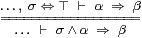
|
By Definition 5.5, “Γ, σ⇔ ⊤” denotes an open subspace of the universe, and “α⇒β” means that one relative open subspace of this is contained in another. Then both lines of the rule on the left say that the intersection of the open subspaces of Γ classified by σ and α is contained in that classified by β.
Because of Definition 4.5, the rule on the right is valid constructively, because it says exactly the same thing as that on the left, except that it concerns the intersection of closed subspaces, cf. the discussion following Definition 3.22.
However, to distinguish our theory of topology from (classical) set theory, we need
Axiom 5.7 Every F:ΣΣ is monotone:
if σ⇒τ then Fσ⇒ Fτ,
cf. Remarks 3.10 and 3.21.
From this we can recover the Phoa principle (Definition 3.22):
Proposition 5.8 Fσ ⇔ F⊥∨σ∧ F⊤. ▫
The Phoa principle will be as important to our logic for topology as the distributive law is to arithmetic. For example, whereas the traditional constructive proof of the intermediate value theorem (Theorem 1.7) requires Dependent Choice, we avoid it in ASD by relying on the Phoa principle (Section 13). More mundanely, we first use it to show that equality in a discrete space obeys the usual properties of substitution, reflexivity, symmetry and transitivity, whilst inequality obeys their lattice duals.
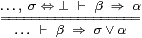
Lemma 5.9
Let N and M be discrete spaces and H and K Hausdorff ones,
let f:N→ M and g:H→ K be functions (Definition 5.3)
and let φ x and ψ x be predicates on N and H
respectively. Then
|
Proof Starting from the basic rule of substitution,
| …, n=m:N ⊢ φ n ⇔ φ m, |
discreteness (Definition 4.7) allows us to replace the statement of equality of terms on the left above by the equality proposition:
| …, (n=N m)⇔⊤ ⊢ φ n ⇔ φ m, |
and then the first rule in Axiom 5.6 transfers this across the ⊢,
| … ⊢ (n=N m)∧φ m=⇒φ n. |
The other results in the left-hand column follow from this.
If you think you understand the results for =, which apply to open subspaces of a discrete space, then you also understand those for ≠, since they say the same thing in the upside-down notation for closed subspaces of a Hausdorff space. Formally,
|
using Definition 4.8 and the second rule in Axiom 5.6. ▫
Whereas the Gentzen rules in topology (together with those for ⇒ in set theory) move propositions across the ⊢, the rules for the quantifiers move a variable. The latter is said to be free in one line of the rule and bound in the other.
Axiom 5.10
The rule for the existential quantifier is
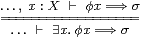
|
in which the propositional expression φ x may contain the variable, but σ must not.
The upward direction of this rule is equivalent to existential instantiation,
| φ a =⇒ ∃ x.φ x. |
The downward direction justifies the mathematical idiom there exists, in which, when given ∃ x.φ x , we may temporarily assume that we have an x that satisfies φ x , in order to deduce any conclusion σ, so long as σ doesn’t depend on what x is. However, no choice is involved in doing this, because the formal rule may be shown to agree precisely with the informal idiom [Tay99, §1.6]. On the other hand, we must not export the value of the witness from the argument.
Remark 5.11
Quantification is the logical form of the infinitary unions in topology,
but arbitrary unions were
the reason why Proposition 2.12 missed the point
of Theorem 2.5,
and more generally of computation (Remark 3.23).
The rule above is therefore not asserted in general in ASD:
the type X of the quantified variable x must be overt.
As far as the familiar spaces in topology are concerned, this is not a severe handicap, since ℕ, ℚ, ℝ and the other base types that we listed in Axiom 4.1 are all overt. The one significant exception that will arise in this paper is that closed subspaces need not in general be overt (Section 16).
Besides the topological properties that we discuss in this paper, the existential quantifier is also employed for combinatorial purposes, even in analysis. For example, we shall want to say that there exists a step function that approximates an integral sufficiently accurately (Remark 10.12). Since this means that there exists a number of steps, as well as that there exist values for each of them, we are quantifying over a more complicated space, to which we shall return in Remark 12.16.
We study overt (sub)spaces more fully in Section 11: the reason for introducing the quantifier here is that we need it to state some of the basic properties of ℕ and ℝ.
Lemma 5.12 The quantifier ∃ is related to ∧
by the Frobenius law,
| τ ∧ ∃ x.φ x ⇔ ∃ x. (τ∧φ x). |
Proof Each side of this law is related to the judgement …,x:X,τ⇔⊤⊢φ x⇒σ by Axioms 5.6 and 5.10. The name is due to Bill Lawvere. ▫
Lemma 5.13
The order < on ℝ admits interpolation
and extrapolation:
| (x< z) ⇔ ∃ y. (x< y)∧(y< z) and ⊤ ⇔ ∃ x z.(x< y)∧(y< z). |
Proof [⇒] by existential instantiation, with y≡½(x+z),
x≡ y−1 and z≡ y+1.
[⇐] by the other direction of Axiom 5.10. ▫
In the same way, from Lemma 5.9, we deduce
Lemma 5.14
For any propositional expression φ x on an overt discrete space N,
| φ n ⇔ ∃ m:N. φ m ∧ (n=N m). ▫ |
Theorem 8.13 gives the dual rules for the universal quantifier ∀, which ranges over a compact space, and Lemma 8.14 is the dual of Lemma 5.14.