


Returning from logic to topology, recall from Definition 1.5 that we need to represent points, open subobjects and compact subobjects in our calculus. These will be given by terms of type X, ΣX and ΣΣX respectively, but whilst the first two correspond exactly, the question of which second order terms denote compact subspaces is more complicated.
We pick up the treatment of compact objects from Section C 7, and show how this leads to the representation of compact subobjects as quantifiers or modal operators. Following [HM81], these should preserve finite meets and directed joins, but the basic idea of ASD is that the directed joins come for free. A compact subobject is therefore represented by a term A:ΣΣX for which A⊤⇔⊤ and A(φ∧ψ)⇔ Aφ∧ Aψ.
This abstract idea works very well as far as the relationship between compact and closed subspaces of a compact Hausdorff space. But then we run into some trouble, because at that point we actually need to use Scott continuity, but our logical structure will not be strong enough to do this until Section 9. There is an alternative treatment in [J] that avoids this problem by restricting to the Hausdorff case, and in particular ℝ and ℝn; you may prefer to read that instead of this section, or in parallel with it.
In the experimental spirit, we try to go further down the path laid by [HM81, JS96], but we stumble into more and more potholes, showing how much more work needs to be done in ASD to make it into a full theory of general topology. But Jung and Sünderhauf do have something interesting to show us when we make this excursion, namely a very close duality between compact and open subobjects of stably locally compact objects.
The abstract analogue of the way in which locale theory treats local compactness is much simpler than this. In that case any term A:ΣΣX may be used — it doesn’t have to preserve meets.
Remark 5.1
Traditionally2,
a topological space K has been defined to be
compact if every open cover,
i.e. family {Us ∣ s∈ S} of open subspaces such that K=⋃s Us,
has a finite subcover, F⊂ S with K=⋃s∈ F Us.
If the family is directed (Definition 1)
then F need only be a singleton,
i.e. there is already some s∈ S with K=Us.
The Scott topology on the lattice |ΣK| offers a simpler way of saying that K is compact. In this lattice, ⊤ denotes the whole of K, so compactness says that if we can get into the subset {⊤}⊂|ΣK| by a directed join ⋃s↑ Us then some member Us of the family was already there3. In other words, {⊤}⊂ΣK is an open subset in the Scott topology on the lattice.
Definition 5.2 In abstract Stone duality we say that
an object K is compact if there is a pullback
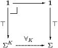
Using the fact that Σ classifies open subobjects (Remark 3.2), together with its finitary lattice structure (but not the Scott principle), Proposition C 7.10 shows that ∀K exists with this property iff it is right adjoint to Σ!K (where !K is the unique map K→1). It is then demonstrated that this map does indeed behave like a universal quantifier in logic (the corresponding existential quantifier was given by Definition 4.3).
Lemma 5.3 If K and L are compact objects then K+L
is also compact, as is ∅.
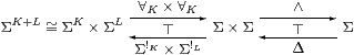
Proof ∀K+L(φ,ψ)⇔∀Kφ∧∀Lψ and ∀∅=⊤:Σ∅≅1→Σ. ▫
The following result is the well known fact that the direct image of any compact subobject is compact (whereas inverse images of open subobjects are open).
Lemma 5.4
Let K be a compact object and p:K↠ X be Σ-epi4,
i.e. a map for which Σp:ΣX→ΣK is mono.
Then X is also compact, with quantifier ∀X=∀X·Σp.
Proof The given quantifier, Σ!K⊣∀K, satisfies the inequalities
| id ≤ ∀K·Σp·Σ!X = ∀K·Σ!K |
| Σp·Σ!X·∀K·Σp = Σ!K·∀K·Σp ≤ Σp, |
from which we deduce Σ!X⊣∀K·Σp, since Σp is mono. ▫
What becomes of the quantifier ∀K when K no longer stands alone but is a subobject of some other object X? We see that any compact subobject K⊂ X defines a map A:ΣX→Σ or A:ΣΣX that preserves ⊤ and ∧. We shall call this a necessity (▫) modal operator, rather than a quantifier, since we have lost the instantiation or ∀-elimination rule Aφ⇒φ x.
Lemma 5.5 Let i:K→ X be any map, with K compact.
Then A≡∀K·Σi:ΣX→Σ preserves ⊤
and ∧.
Moreover Aφ≡∀K(Σiφ)⇔⊤ iff Σiφ=⊤K.
Proof Σi preserves the lattice operations and ∀K is a right adjoint. ▫
Remark 5.6 In traditional language, for any open set U⊂ X
classified by φ:ΣX, the predicate Aφ says whether K⊂ U.
Just as ∀K:ΣK→Σ classifies {⊤}⊂ΣK,
the map A:ΣX→Σ classifies a Scott-open family F
of open subspaces of X, namely the family of neighbourhoods of K.
Preservation of ∧ and ⊤ says that
this family is a filter.
Notice that we have an example of the alternation K⊂ U of compact and open subobjects that we saw in Lemma 1.2. Also, recall from Definition 1.5 that we wanted to test x∈ U and K⊂ U; these are expressed by the λ-applications φ x and Aφ respectively.
Proof
Corollary 5.8 AK⊥⇔⊤ if K is empty, ⊥ if it’s inhabited. ▫
Remark 5.9 Classically, any compact (sub)space that satisfies
AK⊥⇔⊥ must therefore contain a point, by excluded middle,
but Choice is still needed to find it
[Joh82, Exercise VII 4.3].
In the localic formulation, it is a typical use of the maximality principle
to find a prime filter containing F,
so A≤ P in our notation. ▫
The situation in which open and compact subobjects interact extremely well is that of a compact Hausdorff object (Definitions 4.2 and 5.2).
Lemma 5.10 Let X be a compact Hausdorff object and φ:ΣX. Then
|
Proof These are the lattice duals of (x=y)∧φ x ⇔ (x=y)∧φ y, φ x ⇔ ∃ y.(x=y)∧φ y, reflexivity, symmetry and transitivity in any overt discrete object, and the following proof is just the dual of that in Lemma C 6.7.
The closed subobject Δ:X⊂ X× X is co-classified by (≠X), so the corresponding nucleus, in the senses of both locale theory (j≡Δ*·Δ*) and of abstract Stone duality (E≡∀Δ·ΣΔ, Axiom 3.3(c) and Lemma 3.8) takes
| φ:ΣX× X to λ x y.(x≠ y)∨φ y. |
Consider in particular ψ≡Σp0φ, or ψ(x,y)≡φ x; then
| ∀Δφ = ∀Δ·ΣΔ·Σp0φ = ∀Δ·ΣΔψ = (∀Δ⊥)∨Σp0φ. |
The same thing in λ-calculus notation, and its analogue for p1, are
| (∀Δφ)(x,y) ⇔ (x≠ y)∨ φ x ⇔ (x≠ y)∨ φ y. |
Now apply ∀p0≡∀ y, so φ = ∀p0·∀Δφ = ∀p0(∀Δ⊥∨Σp0φ), i.e. φ x ⇔ ∀ y.(x≠ y)∨φ y . Inequality is irreflexive by definition. We deduce symmetry by putting φ≡λ u.(y≠ u) and the dual of the transitive law with φ≡λ u.(u≠ z). ▫
The idea of the following construction is that K⊂ U iff U∪ V=X, and conversely x∈ V iff K⊂ X∖{x}, where K is compact and V is its complementary open subobject, encoded by A and ψ respectively. The lattice dual of this result — that open and overt subobjects coincide in an overt discrete object — was proved for ℕ in Section A 10.
Proposition 5.11 In any compact Hausdorff object K,
there is a retraction ΣK◁ΣΣK given by
|
where, if A is so defined from ψ then it preserves ⊤ and ∧.
Later we shall show that closed and compact subobjects agree exactly.
Proof ψ↦ A↦λ x.A(λ y.ψ y∨ x≠ y)=ψ, by the second part of the Lemma. Then A⊤⇔⊤ easily, whilst A(φ1∧φ2)⇔ Aφ1∧ Aφ2 by distributivity.
On the other hand, A↦ψ↦λφ.∀ x.A(λ y.φ y∨ x≠ y), whilst the first part of the Lemma says that A=λφ.A(λ y.∀ x.φ y∨ x≠ y), so for the bijection between closed and compact objects we need A to commute with ∀ x. To show this, we need to know about the Tychonov product topology on X× X (Remark 8.3), and to use Scott continuity (Theorem 9.6). ▫
As we said, it is not obligatory that the As that we shall use to define locally compact objects in the next section actually satisfy these conditions, i.e. preserve ⊤ and ∧. Consider the localic situation.
Example 5.12 For β∈ L in a continuous lattice
(Definition 3), the subset
| ↑β ≡ {φ ∣ β≪φ} ⊂ L |
is Scott-open, and therefore classified by some A:ΣL (Remark 3.2). However, ↑β need not be a filter (cf. Definition 2.9), so A need not preserve ⊤ or ∧. ▫
We obtain similar behaviour even in traditional topology. The following may seem a strange thing to do, but it will fall into place as we start to use the λ-calculus.
Notation 5.13
In [A] we found it useful to regard any map
F:ΣX→ΣY (not necessarily a homomorphism for the monad
or of frames, but nevertheless Scott-continuous) as a “second class”
map F:Y−× X,
and to write HS for the category composed of such maps.
The work cited there explains how they interpret “control effects”
such as jumps in programming languages.
We shall in particular meet I:ΣX→ΣY
such that Σi· I=id, where i:X↣ Y.
Remark 5.14 Just as in Lemma 5.5
we formed the modal operator corresponding to the direct image i K
of K along i:K→ X as the composite A=∀K·Σi,
so we may form the direct image F A
along a second class map F:K−× X as ∀K· F.
Its open neighbourhoods are given, as in Remark 5.6, by
| ( |
| K⊂φ) ⇔ (∀K· F)φ ⇔ A(Fφ) ⇔ (K⊂ Fφ). |
However, ∀K· F need only be a filter when F preserves ⊤ and ∧.
Even when A does preserve meets, and so classifies a Scott-open filter of open subspaces, it need not correspond to a (locally) compact subspace. (It does in a compact Hausdorff object, but even there we do not yet have to tools to prove it, cf. Proposition 5.11.) We make a brief excursion into classical topology to illustrate the duality of open and compact subspaces, and their alternating inclusions (Notation 1.3). Recall from Definition 1.1 that any open subspace is the union of the compact subspaces inside it: the first result answers the dual question of when a compact subspace is the intersection of the open subspaces that contain it.
Lemma 5.15 Using excluding middle in classical topology
[HM81, p221 def 2.1],
| {y∈ X ∣ ∃ x∈ K.x≤ y} = ⋂↓{U⊂ X open ∣ K⊂ U}, |
where ≤ is the specialisation order (Definition 3.7). We call this the saturation of K. Hence compact subspaces of X can be recovered from their modal operators iff X is T1 (when ≤ is trivial). For a specific non-example, let X≡Σ and K≡{⊥}, so A≡λφ.φ⊥ and the saturation of K is Σ. ▫
What we might hope to recover from the modal operator A, therefore, is the saturation of K, as Karl Hofmann and Michael Mislove did for sober spaces [HM81, Theorem 2.16], and Peter Johnstone did for locales [Joh85]. This result shows that we have identified enough of the properties of modal operators, at least in the classical model.
Lemma 5.16 Let F⊂|ΣX| be a Scott-open
filter of open subspaces of a sober (but not necessarily locally
compact) space. Then, assuming the axiom of choice,
K≡⋂↓F⊂ X is a compact subspace,
and F={U ∣ K⊂ U}. ▫
Lemma 5.17
[HM81, p221 thm 2.16]
Let K≡⋂↓s Ks
be a co-directed intersection of compact saturated subspaces of a sober space.
Then K is also compact saturated, and AK=⋁↑ AKs.
If all of the Ks are inhabited then so is K. ▫
Theorem 5.18
[Kel55, Problem 5 F(a)]
Compact saturated subspaces of a locally
compact sober space form a continuous preframe under reverse inclusion.
That is, for any compact saturated subspace K⊂ X,
| K = ⋂↓{L compact saturated ∣ L≺≺ K}. |
Here L≺≺ K means that there is an open subspace U with K⊂ U⊂ L (sic — Notation 1.3), but this is equivalent to L≪ K, the order-reversed analogue of Definition 2, i.e.
| K ⊃ ⋂↓s Ms ⇒ ∃ s. K⊃ Ms. ▫ |
Corollary 5.19
Using Choice in classical topology,
stably locally compact sober spaces enjoy the dual Wilker property
(cf. Lemma 1.10):
if K∩ L⊂ U then there are open subspaces V and W
and compact ones K′ and L′ such that
K′∩ L′⊂ U, K⊂ V⊂ K′ and L⊂ W⊂ L′
[JS96, Theorem 23].
Proof Use Lemma 2.7 in the continuous lattice of compact saturated subspaces under reverse inclusion. It is significant in this that the abstract joins in the lattice be given by intersections of subspaces. ▫
Remark 5.20 There is still a problem.
Even when X itself is locally compact,
and we have a filter F that is Scott-open and therefore classified
by a term A of type ΣΣX,
the compact subspace K that they define need not be locally compact.
Therefore they need not be definable as actual objects
in the theory that we describe in this paper.
However, an extension to and beyond the category of all locales is envisaged
for later work.
Preliminary investigations in this suggest
that any A:ΣΣX that preserves ⊤ and ∧
can be expressed as the universal quantifier of a compact subobject.
However, as we said at the beginning of this section, the “dual bases” that we shall introduce in the next section use the As and not the Ks. It is a desirable property of A that it be a filter, i.e. preserve ⊤ and ∧, because then we can fully exploit the intuitions of traditional topology. But it is not necessary: locale theory gives rise to bases that don’t have this property, and both ways of doing things have their advantages.