


Since the work [H] on which this section is based was stalled, I need to look at it again to check certain assertions below.
In this section we consider an additional axiom that has the effect of turning the full subcategory of overt discrete spaces from a pretopos into an elementary topos. This allows us to compare ASD more closely with the textbook theories of topology that are based on set theory or toposes.
Since the new structure is not computable, it is a diversion from our main goal of formulating computable topology — I believe that the important features of general topology only depend on computable foundations. Nevertheless, it is methodologically important, because it shows which features of traditional topology we must sacrifice in the computable account.
The details behind this section may be found in [H]. It offers one way in which the ideas of ASD might be extended beyond locally compact spaces, but there are currently no models apart from LKLoc with which to compare them. Nor is is clear whether this extension is compatible with the one that we discuss in §12.
10.1.
Recall that the category BbkSp of Bourbaki spaces is related to the category of sets by the adjunctions
in the diagram on the left,
in which the downward functor yields the underlying set of points of
a space and its adjoints equip any set with its finest and coarsest topologies.
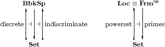
Considered as a frame, the powerset of a set provides its discrete topology, and therefore the left adjoint in the second diagram. Notwithstanding the fact that locales need not have enough primes (§4.2) or points [Joh82, §II 1.3] to make the functor faithful, the set of them gives the right adjoint. However, there is no such thing as the “indiscriminate” topology in locale theory, since by definition any locale has exactly the points that are determined by its open sets.
Topological spaces are axiomatised intrinsically in ASD, but could they possibly have “underlying sets” in a sense like this? As we explained in the previous section, overt discrete spaces play the role of sets, so the inclusion Δ:E⊂S of this full subcategory corresponds to the “discrete topology” functor above.

In this section, therefore, we assume that this inclusion has a right adjoint U, called the underlying set functor. Since the objects of ASD, like locales, are all sober, there is no indiscriminate topology.
Recall our convention that N and M denote overt discrete objects.
10.2. What is the underlying set of the Sierpinski space Σ
or of the topology ΣN?
As we might expect from §§7.5 & 5.4,
they are respectively the subobject classifier Ω
and powerset ΩN of N in E.
In particular, E is a topos.
The subcategory E⊂S is closed under finite limits, including 1, products, equalisers, pullbacks and monos. Also, any mono in E, being a map from an overt object to a discrete one, is an open inclusion (§7). Hence any binary relation from N to M in E, i.e. a mono i:R↪ N× M, is classified by φ:N× M→Σ in S, as in the diagram on the left.
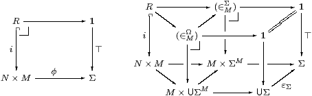
This square factorises into the two pullback squares at the back of the diagram on the right; As the functor U preserves pullbacks, it takes the squares at the back of the diagram to those on the left and front (from R to UΣ). Hence
| (∈MΩ) ≡ U(∈MΣ) ↪ M×UΣM |
is the generic binary relation on M, as required to make E a topos.
The object U(ΣM) has the universal property of the exponential ΩM within E, i.e. when we test it with maps N→U(ΣM) from overt discrete objects. However, this does not extend to general test objects in S, and for this reason we prefer to write Ω M≡U(ΣM) instead of ΩM.
10.3.
For reasons that we shall explain in §10.8,
we say that an object X∈S has
The converse to the result of the previous paragraph is that, if E is a topos then there is a partial right adjoint U that is defined on those objects that have enough opens.
10.4. We want to compare ASD with other theories of topology.
The latter, i.e. the categories of frames, locales, locally compact locales
and so on, can be constructed over any topos, such as E,
in essentially the same way as they are defined over sets.
We can even pretend that our E is Set, so long as
we understand “set theory” to mean the structure of an elementary topos.
Our category S can also be treated in this way, because it is
E-enriched, i.e. its “homs” S(X,Y) can be given the
structure of objects of E.
The difference between ASD and the other theories is that
For example, ⊑ (§8.2) is intrinsic to ΣX, but the arithmetical order ≤ is imposed on ℕ (§9.5). Notwithstanding its universal property, the structure on the object Ω, including ¬ and ⇒, is imposed in this sense (§10.7).
The objective is to show that the whole of our category S is equivalent to some category that is (re)constructed from objects of the subcategory E.
10.5.
We may compare S with categories such as Loc that are defined over E.
Consider the adjunctions amongst Sop, S and E
that are given by the monadic framework (§6)
and the underlying set hypothesis (§10.1), as shown on the left:
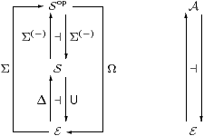
It is convenient to write Σ⊣Ω for the composite functors. These induce a monad on E, so let A be its category of Eilenberg–Moore algebras, and there is a comparison functor Sop→A.
Even though Sop⇄S was assumed to be monadic, the composite need not be, i.e. the functor Sop→A need not be an equivalence. It is, however, full and faithful in the case where every object of S is definable in the monadic framework . This happens, for example, when S is the category of locally compact locales (§5.10).
In general, this functor need only identify a full subcategory of S with one of Aop. The former consists of the spaces that have enough opens (§10.3), but further hypotheses are needed to fix the latter. In particular, we need Scott continuity to say that the monad on the topos E agrees with the one for Frm (§§4.4 & 11.8).
10.6.
The symbolic formulation of the underlying set functor is one of the
clearest examples of translating an adjunction into a system of
type-theoretic rules (§2.11).
For any type X∈S, we have

|
| Γ⊢ε(τ. a)=a:X and x:U X ⊢ x=(τ.ε x):U X. |
In short, τ. may be applied to any term so long as all of its free variables are of overt discrete type. In other words, it allows variation over a “combinatorial” structure but not a “geometrical” one.
10.7.
The overt discrete object Ω carries imposed operations
(⋏, ⋎, ≤) that make it a distributive lattice.
These are just the U-images of the homologous intrinsic operations
(∧, ∨, ⇒) on Σ,
which remain nullary and binary on Ω
because U (being a right adjoint) preserves products.
In particular, (≤):Ω×Ω→Σ,
cf. equality for discrete spaces in §§8.6 & 9.3.
But unlike Σ, Ω also has the imposed structure of a complete Heyting algebra, as does the set (E-object) Ω X≡U(ΣX) of opens of any space X, where (⇒):Ω X×Ω X→Ω X is defined by
| (φ⇒ψ) ≡ τ.λ x:X.∃θ:UΣX. εθ x ∧ (φ⋏θ≤ψ) |
and ⋁:ΣΩ X→ΣX by
| ⋁ F ≡ λ x:X.∃θ:UΣX. Fθ∧ (εθ)x. |
Moreover, for any map f:X→ Y in S, we have f*⊣ f* with respect to the imposed order inherited from Ω, where
| f*ψ ≡ Ω f ≡ τ.λ x:X.(εψ)(f x) |
and
| f*φ ≡ τ.λ y:Y. ∃θ:UΣY. (εθ)y∧(f*θ≤φ). |
10.8.
Using this notation, we can ask whether the intrinsically continuous
functions in the category S that we have axiomatised directly agree
with the imposed structure of the categories of locales and Bourbaki
spaces over the topos E.
If we are given an S-morphism g:X→ Y,
the maps f≡U g and H≡ g* make the two squares commute:
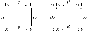
Conversely, if X has enough points (εX:U X→ X is epi, §10.3) then εX*:Ω X↣ΩU X is split mono, so Ω X is a sublattice of the powerset of the underlying set of X, as in a Bourbaki space.
Then we may say that a function f between the underlying sets is continuous in the imposed (Bourbaki) sense if there is a map H that makes the square on the right commute. If X has enough points and Y has enough opens (§10.3) then f and H arise from some unique S-map g.
Once again, we have a lot of structure that looks like topology, even though we have said nothing to ensure that the category A of “algebras” in §10.5 is actually that of frames over E. The relevant condition is one of the formulations of Scott continuity that we consider in the next section (§11.8). The result is that the full subcategory of spaces with enough points and enough opens is equivalent to the category of sober Bourbaki spaces over E, and the whole category of Bourbaki spaces is equivalent to a full subcategory of the comma category E↓S.
We shall not assume the underlying set axiom in the remainder of this paper.