


Whereas there is only one notion of “subset” in set theory, in topology we need to distinguish between open and other kinds of subspaces . Besides this, open subspaces are used in two different ways in our arguments: not only as particular spaces that are included in larger ones, but also as generic tests that are used in the definition of compactness. This section introduces our notation for these two roles: we use the λ-calculus for open subspaces considered as tests, and adopt {} from set theory for inclusions of general subspaces.
We will set out the λ-calculus in a relatively formal way because, as we said in Remark 5.1, logic thereby undertakes the burden of proof of continuity. Because of the methods that we sketched in Section 3, any well formed expression in our language denotes a function that is automatically continuous in traditional general topology. Our purpose in this paper is to show that it is possible to do some things in elementary real analysis entirely within this language. Traditional set-based topology is then redundant, because we (or a machine) may compute directly with our language, so we have made the first step towards using computation instead of set theory as the foundations for analysis.
Remark 7.1 Recall from Section 3 that open subspaces of X
correspond uniquely to continuous functions X→Σ,
so the topology on X is the collection of such functions.
However, we do not consider this as a set
but as another space, which we call ΣX;
in traditional terms, it carries the Scott topology.
The meaning of ΣX is captured by Theorem 3.19:
there is a bijection between continuous functions
| Γ× X —→ Σ and Γ—→ ΣX. |
This is the recursion step in the proof that every well formed expression denotes a continuous function in traditional topology. We may re-state it as
Proposition 7.2
If the denotation (in the sense of Definition 5.5) of
| Γ, x1:X1,…,xn:Xn ⊢ σ is a continuous function ⟦Γ⟧×⟦X1⟧×⋯×⟦Xn⟧ —→Σ |
then the denotation of
| Γ ⊢ λ x1… xn.σ is a continuous function ⟦Γ⟧—→ Σ⟦X1⟧×⋯×⟦Xn⟧, |
where the products are given the usual Tychonov topology and Σ⟦X1⟧×⋯×⟦Xn⟧ the Scott topology [Sco72, Section 3]. ▫
Remark 7.3 The typed λ (lambda)-calculus,
which gives a name to the forward correspondence,
may seem to be little more than a change of symbols,
especially when it is used for sets.
In topology, on the other hand,
Theorem 3.19 depends crucially on the correct definitions
of local compactness and of the Scott topology,
so these ideas are built in to the syntax.
Whenever we use this syntax, we therefore implicitly invoke that Theorem.
We intend to use these ideas to define compactness and overtness. We saw in Section 2 that these are captured by operations ▫ and ◊ that preserve directed unions, so are continuous functions ΣX→Σ with respect to the Scott topology. We therefore handle them in our language as terms of this type. Any well formed expression F such as ▫ or ◊ of this type denotes such a continuous function, and so Fφ is of type Σ and denotes a member of the Sierpiński space.
However, in order to discuss terms of higher types like these, we need to be able to treat a function φ:X→Σ as a thing in itself (of type ΣX). This is why we need the typed λ-calculus, instead of the informal ways in which mathematicians usually talk about functions, and which we too have been using so far. There are numerous textbook accounts of λ-calculi and the way in which they, and the β-rule in particular, relate to computation. Beware, however, that they usually talk about arbitrary function-types YX (also written X→ Y), whereas we only allow ΣX and (ΣY)X≅Σ(Y× X). This corresponds to only allowing λ to bind logical expressions. See Section I 4 for how these general treatments are specialised to ASD.
In order to distinguish our own λ-calculus from the generic ones, we need to define its types, its terms and the rules that say when two terms of the same type are to be interchangeable (regarded as equal). Axiom 4.1 listed the base types and the ways of forming new ones that we use in this paper. We have already introduced the terms for the arithmetic of ℕ, ℚ and ℝ and for the logic in Σ, so we need to say how the λ-calculus provides other ways of forming terms.
Axiom 7.4
For any proposition (term of type Σ)
| …, x1:X1,…, xn:Xn ⊢ σ, |
possibly containing variables x1,…,xn of any type and maybe some other variables (or “parameters”) from the list …, we may form the predicate
| … ⊢ λ x1,…, xn.σ, |
in which x1,…,xn are bound by lambda abstraction, but the other variables in the list ⋯ remain free. The type of λ x1,…, xn.σ is X1→⋯→ Xn→Σ or ΣX1×⋯× Xn, where the convention is that X→ Y→Σ means X→(Y→Σ).
Axiom 7.5
Conversely, given any predicate φ of type ΣX1×⋯× Xn
and expressions (“arguments”) a1:X1, ..., an:Xn
of the corresponding types, any of which may contain parameters,
we may apply the predicate to the arguments,
yielding the proposition φ<a1, a2, …, an>.
Application is given by the map ev:ΣX× X→Σ, whose denotation is jointly continuous by Proposition 3.17. Hence, in the backward direction of Theorem 3.19, if the denotations of φ, a1, ..., an are continuous functions then so is that of φ<a1, a2, …, an>. This and Proposition 7.2 are the steps in the proof by recursion that every term denotes a continuous function.
Finally, there are rules to say that the two directions of the correspondence are mutually inverse. We need these in order to be able to reason entirely within the calculus itself, without referring back to the model.
Axiom 7.6
When a lambda-abstraction φ≡λx.σ
is applied to arguments, the result is equivalent to substitution
of those arguments for the abstracted variables:
| (λ x1:X1,…, xn:Xn.σ)<a1, a2, …, an> ⇔ [a1/x1,…,an/xn]*σ. |
This is called the β-rule. Its converse is the η-rule: we recover the given function or predicate if we apply it to fresh variables and then abstract them:
| (λ x1,…, xn.φ x1… xn) = φ, |
this being an equational statement (Definition 4.5) between terms of type ΣX1×⋯× Xn. The β- and η-rules are equivalent to saying that the correspondence in Theorem 3.19 is bijective.
Naturality (in the categorical sense) is captured by
Axiom 7.7
We may substitute a term for a free variable:
| [a/x]*λ y.σ = λ y.[a/x]*σ and [a/x]*(φ b) ⇔ ([a/x]*φ)([a/x]* b), |
so long as x and y are distinct variables and y is not a free variable in a.
Besides equalities of λ-terms such as these, the lattice structure of Σ gives rise to an order relation:
Notation 7.8
If the propositions σ,τ:Σ
with parameters x:X are related by σ⇒τ
or σ⇔τ then (as we have just done)
we write λx.σ⊑λx.τ
or λx.σ=λx.τ for the corresponding
relationships between the predicates.
So ⊑ is really the same as ⇒: we just use two symbols
for clarity, distinguishing between propositions (type Σ) and
predicates (type ΣX).
Now we turn to subspaces in the sense of inclusions, starting with two familiar cases.
Axiom 7.9
The predicates ⊢α,ω:ΣX (without parameters)
give rise to
Plainly we need some notation to distinguish between
these two subspaces that arise from the same predicate.
The curly brackets are no more than convenient symbols and
are in no way intended to be a re-introduction of set theory.
As with other parts of the language,
we must give the rules according to which we may manipulate these symbols.
In particular, any type X in our language is to be regarded, not just as a set of points or terms, but as a space, whose topology is another space, the exponential ΣX. In order to introduce U and C as types, we therefore have to construct ΣU and ΣC too.
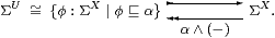
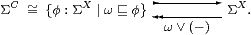
Axiom 7.10
The exponentials ΣU and ΣC are
obtained as retracts of ΣX by splitting the idempotents
α∧(−) and ω∨(−) respectively.
Hence the open subsubspaces of U and C are canonically represented
as those open subspaces φ of X
that lie between the least and greatest ones:
| for U: ⊥U≡⊥X⊑φ⊑⊤U≡α and for C: ⊥C≡ω⊑φ⊑⊤C≡⊤X. |
The intersection of an open subspace with a closed one is written {x ∣ α x & ¬ω x} and called locally closed. It is the result of composing the constructions above (which commute) and its open subsubspaces are represented by φ:ΣX with ω∧α⊑φ⊑α.
On the other hand, if α and ω are complementary (Lemma 6.4) then each of them defines a clopen (both closed and open) subspace.
Remark 7.11 These idempotents arise from the canonical ways of converting
open subspaces of X into those of U and C and conversely.
For an open subsubspace V⊂ U⊂ X, this is easy:
V is already an open subspace of X,
classified by φ with φ⊑α, so
In the closed case, given W⊂ C⊂ X, the union V≡ W∪ U⊂ X is open, where V (not W) is classified by φ:ΣX with ω⊑φ. Hence we have the representation
It is then necessary to show that these retracts of ΣX obey the bijective correspondences
 and
and

|
using the fact that any map on the top row extends to one Γ× X→Σ. The argument within the abstract ASD calculus depends on Axiom 5.6 and is given in [C].
Remark 7.12 This suggests a more general situation,
in which the inclusion i:Y↣ X
is Σ-split by a map I:ΣY↣ΣX
for which Σi· I=id.
In fact, any computably based locally compact space Y
can be represented in this way with X≡Σℕ
[G].
The language for Σ-split subspaces is described in [B] and more briefly in Section I 5. Axioms 7.9 and 7.10 above are special cases of Axioms 5.14 and 5.15 in [I]. Another example (the main subject of [I]) is the Dedekind-cut representation ℝ↣Σℚ×Σℚ, for which the existence of the Σ-splitting is equivalent to the Heine–Borel theorem. However, in this paper we have avoided using the general construction by taking ℝ as a base type and the Heine–Borel theorem as Axiom 9.5.
Besides being complicated to work with, Σ-split subspaces are not really appropriate for the concepts that we wish to discuss here. Any Σ-split subspace of a locally compact space is locally compact, but this need not be true of a compact subspace of a non-Hausdorff locally compact space (or of an overt subspace of a non-discrete one).
The system of types including the constructor Σ(−) cannot be generalised to allow such subspaces if we want to retain an interpretation within traditional general topology, because the exponential ΣX only exists in that category when X is locally compact (Proposition 3.17).
Now, the goal of ASD is to re-axiomatise topology, not the objects that have usurped the name “topological spaces” in the textbooks — larger categories are known in which all exponentials exist. However, the process of adapting these to the principles of ASD is ongoing research that is by no means straightforward and is certainly well beyond the scope of this paper [M].
All that we really need in the rest of this paper is a way of giving names to open, closed, compact and overt subspaces. We shall do this by generalising Axiom 7.9 without 7.10.
Remark 7.13
We shall see that a term Γ⊢ a:X
belongs to one of these kinds of subspaces
if it satisfies a certain equation
f(a)=g(a) between terms of some type Z.
For example, open and closed subspaces are defined by the equations
α x⇔⊤ and ω x⇔⊥ with Z≡Σ,
and we will use Z≡ΣΣX for compact subspaces.
Thus membership means that the composites
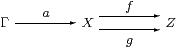
are equal. The subspace that we require is therefore the equaliser of this parallel pair, which is tested by any context Γ, i.e. by terms with parameters and satisfying equational hypotheses. This is general categorical language that in no way depends on either set theory or traditional topology.
The problem with the textbook categories of topological spaces is that locally compact spaces admit the exponentials Σ(−) that we require, but not equalisers, whilst the usual category of “all” spaces has equalisers but not exponentials. In a future, more general, formulation of ASD, we would expect to have both of these, abandoning the traditional categories, but for now we want to retain compatibility.
Definition 7.14 We therefore distinguish between
In Definition 4.5 we introduced the word statement for any equation between terms, whereas we called the terms themselves propositions or predicates if they are of type Σ or ΣX respectively. The inequality φ⊑ψ in Notation 7.8 is also a statement, because it is equivalent to the equation φ∧ψ=φ and also to φ∨ψ=ψ.
Axiom 7.15
A subspace of a space X is defined by putting
a statement p(x) (with no parameters besides x)
on the right of the divider in the notation
| {x:X ∣ p(x)}, |
where p(x) may be φ x⇔ψ x, φ x⇒ψ x, φ x⊑ψ x, f x=g x or a conjunction of these.
Then any term a of type X (which may now contain parameters) is called a member or element of the subspace,
| …⊢ a∈ {x:X ∣ p(x)}, if it satisfies the statement …⊢ p(a). |
We therefore use this notation according to the familiar idiom of comprehension, but its axiomatic force is exactly that the map denoted by a has equal composites with the parallel pair whose equaliser defines the subspace in Remark 7.13.
The denotation of a subspace is the equaliser computed in the traditional category of topological spaces.
Membership or elementhood of a general subspace is therefore another species of statement, whereas that of an open subspace is a proposition. As we intended, the distinction between propositions and statements in logic matches that between open and general subspaces in topology.
Once again we stress that our “comprehension” is not set theory: we have just given the symbolic rules that allow us to introduce and eliminate the symbols {} and ∈, as we did earlier for relations, connectives, quantifiers, descriptions, Dedekind cuts and the λ-calculus. Indeed, for general subspaces, the only situation in which the curly brackets are meaningful is together with the ∈ symbol.
Remark 7.16
In the next section we want to use the subspace notation to prove
that any compact subspace of a Hausdorff spaces is closed.
However, instead of an a priori set-theoretic notion of general subspace that can be closed or compact as a secondary property, Axiom 7.15 provides one construction of a subspace based on the data for compactness, and another based on the idea that it is closed, both by means of equalisers. In other words, we are given the compact and closed subspaces separately, and need to show that they are isomorphic.
However, instead of defining mutually inverse maps between the two objects, there is a categorical technique (with its origins in sheaf theory) known as using generalised elements. These are incoming maps from an arbitrary object Γ of the category. By considering the two objects in each of the roles, this establishes the isomorphism: we just have to show that these incoming maps are in bijection.
The beauty of this method is that it requires exactly the same piece of reasoning as (both the set-theoretic language and also) the symbolic one in our new calculus. By Definition 5.3, an incoming continuous function is a term possibly containing parameters, and the generic such term is a variable.
However, along with the parameters come assumptions (Definition 5.2), so we have
Definition 7.17 For statements p(x) and q(x)
involving only the variable x:X, we write
| {x:X ∣ p(x)} ⊂ {x:X ∣ q(x)} ⊂ X if x:X, p(x) ⊢ q(x) |
and say that one subspace is contained in or a subspace of the other. If both of the containments hold then we say that these subspaces are equal. Similarly, we write
| {x:X ∣ p(x)} ⋂ {x:X ∣ q(x)} ≡ {x:X ∣ p(x) & q(x)} |
for their intersection, where & is the conjunction of statements that we mentioned in Definition 4.5. (The union is a more delicate issue.)
These rules agree with our definition of membership. Hence the subspaces are syntactic sugar: they actually not needed at all, because we can just reason with the language of terms and statements.
In the next section we will begin to use this notation for compact subspaces, but first we apply it to open and closed ones, beginning with an example of Axiom 7.15:
Examples 7.18
For any term a:X, we then have, as in Definition 4.5,
|
We can also show that any function (Definition 5.3) is continuous in the sense that the inverse image of any open or closed subspace is again open or closed respectively.
Definition 7.19
The inverse image of a predicate φ:ΣY
along a function f:X→ Y is given by composition.
There are several notations for this, coming from different disciplines:
| f*φ ≡ f−1φ ≡ Σfφ ≡ (f;φ) ≡ (φ· f) ≡ λ x.φ(f x):ΣX. |
The corresponding open and closed subspaces of X are
| f−1{y:Y ∣ α y} ≡ {x:X ∣ α(f x)} and f−1{y:Y ∣ ¬ω y} ≡ {x:X ∣ ¬ω(f x)}. |
Lemma 7.20
These are indeed the inverse images in a sense that is
consistent with our definitions of membership for a:X:
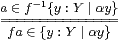 and
and
 ▫
▫
|
Whilst open and closed subspaces have inverse but not direct images under general continuous functions, we shall see in Theorem 8.9 and Notation 11.13 respectively that it is the other way round for compact and overt ones.
Since the traditional categories do not admit all of the structure that we would like, the question of what is the appropriate general notion of topological space remains a matter of debate. We shall therefore only use the subspace notation in a suggestive way, restricting our attention to those compact or overt subspaces that are also (either given or may be shown to be) open or closed.
Since ℝ is Hausdorff, this presents no problem for the compact subspaces that primarily interest us, and the next section unashamedly exploits that simplification. On the other hand, there are overt subspaces that are neither open nor closed, arising from singular ◊-operators (Section 2). However, the worst example that I have been able to find (Remark 16.14) is locally closed and therefore still locally compact.