


The papers on abstract Stone duality may be obtained from
I would like to thank Carsten Führmann, Ivor Grattan-Guiness, Peter Johnstone, Peter Landin, Andy Pitts, John Power, Pino Rosolini, Phil Scott, Hayo Thielecke, Steve Vickers, Graham White, Claus-Peter Wirth and Hongseok Yang for their helpful comments on this paper.
Sober Spaces and ContinuationsPaul Taylor |
Abstract: A topological space is sober if it has exactly the points that are dictated by its open sets. We explain the analogy with the way in which computational values are determined by the observations that can be made of them. A new definition of sobriety is formulated in terms of lambda calculus and elementary category theory, with no reference to lattice structure, but, for topological spaces, this coincides with the standard lattice-theoretic definition. The primitive symbolic and categorical structures are extended to make their types sober. For the natural numbers, the additional structure provides definition by description and general recursion.We use the same basic categorical construction that Thielecke, Führmann and Selinger use to study continuations, but our emphasis is completely different: we concentrate on the fragment of their calculus that excludes computational effects, but show how it nevertheless defines new denotational values. Nor is this “denotational semantics of continuations using sober spaces”, though that could easily be derived.
On the contrary, this paper provides the underlying λ-calculus on the basis of which abstract Stone duality will re-axiomatise general topology. The leading model of the new axioms is the category of locally compact locales and continuous maps.
| Contents | 6 | Enforcing sobriety | ?? | |||
| 1 | Computational values | ?? | 7 | The structure of SC | ?? | |
| 2 | The restricted λ-calculus | ?? | 8 | A lambda calculus for sobriety | ?? | |
| 3 | Algebras and homomorphisms | ?? | 9 | Theory of descriptions | ?? | |
| 4 | Sobriety and monadicity | ?? | 10 | Sobriety and description | ?? | |
| 5 | Topology revisited | ?? | 11 | Directions | ?? |
[This paper is the first part of the core theory of Abstract Stone Duality for locally compact spaces. It appeared in Theory and Applications of Categories 10, pages 248–299, in July 2002, but this version includes some minor corrections. Note also that the analogue of the connection between sobriety and definition by description for ℕ is Dedekind completeness for ℝ [I].]
What does it mean for a computation to yield a value?
If the computational object is a function, or a database measured in terabytes, we may only obtain parts of its value, by querying it with arguments or search-terms. It is usual to say that if the type of the object is simple then the object is directly observable, but for complex types we must perform some computational experiment in order to access the value.
Typically, ℕ is regarded as an observable type [Plo77], but, as Alan Turing had already observed [Tur35, Section 8], if we are given two numbers with a lot of digits, say 9999999999999999 and 999999999999999, we may only determine whether or not they are equal by carefully comparing them digit by digit. For very large numbers, it may not even be feasible to print out all of the digits, so we are back in the situation of merely being prepared to print (or, indeed, to compute) whichever of the digits are actually required. Recursion theory traditionally regards the contents of a database as a huge number too.
So much for integers. What does it mean to define a real number? It is no good writing it out in decimal notation — even overlooking the ambiguity between 0.99999... and 1.00000... — because such an expression is necessarily finite, and therefore defines a rational number. For me to give you a real number in this notation, you have first to tell me how many decimal digits you require.
This interactive manner of obtaining mathematical values goes back to Weierstrass’s definition of continuity of f:ℝ→ℝ at u,
| ∀є> 0.∃δ> 0.∀ u′. |u′−u|<δ⇒|f(u′)−f(u)|<є. |
We ask the consumer of f(u) how much accuracy (є) is required, and pass this information back to the producer of u as our own demand (δ) on the input.
Remark 1.1 In all of these examples, the value can only be elucidated by
being ready to use it in situations that ultimately result in an
observable value. In general, the best I can do is to be prepared
(with a program) to provide as much information as you actually require.
The theme of this paper is that, once we have loosened our control over computational values to this extent, we open the floodgates to many more of them.
As ℕ is too big a type to be observable, maybe we should use 2, the type of bits? But no, this assumes that all computations terminate, so we need a type that’s simpler still. The type Σ of semi-bits is the only observable type that we need: such a value may be present (“yes”), or may never appear (“wait”). Σ is like the type that is called unit in Ml, but void in C and Java. A program of this type returns no useful information besides the fact that it has terminated, but it need not even do that. The results of many such programs may be used in parallel to light up a dot-matrix display, and thereby give an answer that is intelligible to humans.
Remark 1.2
Abstractly, it is therefore enough to consider a single program
of type Σ, so long as we allow processing to go on in parallel.
A computation φ[x] of type Σ is an affirmative property of x, that is, a property that will (eventually) announce its truth, if it is true. Steven Vickers has given a nice account of properties that are affirmative but false, refutative but true, etc., showing how the algebra of affirmative properties has finite conjunctions and infinitary disjunctions, just like the lattice of open subsets of a topological space [Vic88, Chapter 2].
Indeed, by running two processes in parallel and waiting for one or both of them to terminate, this algebra admits binary conjunction and disjunction, whilst there are trivial programs that denote ⊥ and ⊤. The other possibility is to start off (one at a time) a lot of copies of the same program, giving them each the input 0, 1, 2, ..., and wait to see if one of them terminates. If the nth program terminates after N steps, we ignore (silently kill off) the n+N−1 other processes that we have started, and don’t bother to start process number n+N+1 that’s next in the queue to go. This existential quantifier is similar to the search or minimalisation operator in general recursion, though in fact it is simpler, and general recursion can be defined from it.
Definition 1.3
Mathematically, these constructions make Σ into a
lattice with infinitary joins, over which meets (⊤,∧) distribute.
It is convenient to consider finite (⊥,∨) and directed (⋁↑)
joins separately.
Allowing joins of arbitrary families, as is required in
traditional point-set topology, such a lattice is called a frame.
For computation, the joins must be recursively defined, and in particular countable. It is one of the objectives of the programme (Abstract Stone Duality) to which this paper is an introduction to re-formulate topology to agree with computation.
Because of the halting problem, there is no negation or implication. Nor is a predicate of the form ∀ n:ℕ.φ[n] affirmative, as we never finish testing φ[n]s. Whilst we can use proof theory to investigate stronger logics, we can only talk about them: the connectives ∧ and ∨, and the quantifier ∃ n, constitute the logic that we can do. In particular, we can do the pattern-matching and searching that proof theory needs by using ∧, ∨ and ∃.
We write ΣX for the type (lattice) of observations that can be made about values of type X, because λ-abstraction and application conveniently express the formal and actual roles of the value in the process of observation. Observations, being computational objects, are themselves values that we can access only by making observations of them. The type of meta-observations is called ΣΣX, and of course there are towers of any height you please.
There is a duality between values and observations.
Remark 1.4
One special way of making a meta-observation P:ΣΣX
about an observation φ:ΣX
is to apply it to a particular value p:X.
We write
| P ≡ ηX(p) for the meta-observation with P(φ) ≡ φ(p). |
Thus P is a summary of the results φ(p) of all of the (possible) observations φ that we could make about p. (Being itself a computational object, the value of P can only be accessed by making observations ...)
If someone gives us a P, they are allegedly telling us the results of all of the observations that we might make about some value p, but to which they are giving us no direct access. Must we accept their word that there really is some value p behind P?
First, there are certain “healthiness” conditions that P must satisfy [Dij76, Chapter 3]. These are rather like testing the plausibility of someone’s alibis: was it really possible for someone to have been in these places at these times?
Remark 1.5
The application of observations to a value p respects the lattice
operations on the algebra of observations:
Hayo Thielecke calls values that respect these constant observations discardable, though the point is that it is safe to calculate them, even when we may not need to use them.
See also [Smy94, Section 4.4] for further discussion of the relationship between non-determinism and the preservation of lattice structure.
Examples 1.6
Here are some programs that violate the properties above,
i.e. which respectively fail to preserve the logical connectives on the left,
although we are mis-using “the” here (Section 9).
|
Definition 1.7
A subset P of a frame is called a filter
if it contains ⊤, it is closed upwards,
and also under finite meets (∧).
A completely coprime filter is one such that,
if ⋁ U∈ P, then already u∈ P for some u∈ U.
Classically, the complement of such a filter is a prime ideal, I,
which is closed downwards and under infinitary joins,
⊤∉ I, and if u∧ v∈ I then either u∈ I or v∈ I.
Remark 1.8
The motivations that we have given were translated from topology,
using the dictionary [[Smyth?]]
| point | value |
| open subset | observation |
| open neighbourhood | observation of a value. |
This view of general topology is more akin to Felix Hausdorff’s approach [Hau14] in terms of the family of open neighbourhoods of each point than to the better known Bourbaki axiomatisation of the lattice of all open subsets of the space [Bou66]. Beware that we only consider open neighbourhoods, whereas for Bourbaki any subset is a neighbourhood so long as it contains an open subset around the point. Bourbaki writes B(x) for the collection of such neighbourhoods of x.
Remark 1.9 The family P=ηX(p) of open neighbourhoods of a point p∈ X
is also a completely coprime filter
in the frame ΣX of open subsets of X:
Remark 1.10 In Theorem 5.12
we make use of something that fails some of these conditions,
namely the collection {U ∣ K⊂ U} of open neighbourhoods
of a compact subspace K⊂ X.
This is still a Scott-open filter (it respects ⊤, ∧ and ⋁↑),
but is only coprime if K is a singleton.
(At least, that is the situation for T1-spaces: the
characterisation is more complicated in general. When we use this
idea in Theorem 5.12, K must also be an upper subset
in the specialisation order.)
Remark 1.11
So far we have only discussed computations that run on their own,
without any input.
In general, a program will take inputs u1:U1, ..., uk:Uk
over certain types, and we conventionally use Γ to name
this list of typed variables. For the moment, we take k=1.
Suppose that P(u):ΣΣX is a meta-observation of type X that satisfies the conditions that we have described, for each input value u∈ U. If φ:ΣX is an observation of the output type X then P(u)(φ) is an observation of the input u, which we call ψ(u)≡ H(φ)(u). Then the lattice-theoretic properties of P(u) transfer to H:
|
together with the infinitary version, H(⋁↑φi)=⋁↑ H(φi).
So computations are given in the same contravariant way as continuous functions are defined in general topology.
Remark 1.13 Since we only access values via
their observations,
This is a Leibniz principle for values. The corresponding property for points and open subsets of a topological space is known as the T0 separation axiom. An equality such as φ[a] ⇔ φ[b] of two terms of type Σ means that one program terminates if and only if the other does. This equality is not itself an observable computation, as we cannot see the programs (both) failing to terminate.
Remark 1.14
Now suppose that the system P of observations does satisfy the
consistency conditions that we have stated, i.e. it is a completely
coprime filter.
Must there now be some point p∈ X such that P=ηX(p)?
In the parametric version, every frame homomorphism H:ΣX→ΣU is given by Σf for some unique continuous function f:U→ X. [Sobriety means existence and uniqueness.]
We shall show in this paper that the lattice-theoretic way in which we have introduced sobriety is equivalent to an equational one in the λ-calculus. In Section 9 we return to a lattice-theoretic view of ℕ, where the corresponding notion is that of a description, i.e. a predicate that provably has exactly one witness. Then sobriety produces that witness, i.e. the number that is defined by the description. Taking the same idea a little further, we obtain the search operation in general recursion.
In topology, sobriety says that spaces are determined (up to isomorphism) by their frames of open subsets, just as points are determined (up to equality) by their neighbourhoods. Sobriety is therefore a Leibniz principle for spaces. The next step is to say that not only the spaces but the entire category of spaces and continuous functions is determined by the category of frames and homomorphisms — a Leibniz principle for categories. This is developed in [B], for which we set up the preliminaries here.
Another idea, called repleteness, was investigated in synthetic domain theory [Hyl91, Tay91]. This played the same role in the theory as sobriety (cf. Remark 10.9), but it is technically weaker in some concrete categories.
Remark 1.15 We have stressed that a meta-observation P:ΣΣX
only defines a value of type X when certain conditions are satisfied.
Indeed, we justified those conditions by excluding certain kinds
of programs that have non-trivial computational effects.
Since fire burns, we adopt precautions for avoiding it or putting it out — that is the point of view of this paper. On the other hand, fire is useful for cooking and heating, so we also learn how to use it safely.
The mathematical techniques discussed in this paper are closely related to those that have been used by Hayo Thielecke [Thi97a, Thi97b], Carsten Führmann [Füh99] and Peter Selinger [Sel01] to study computational effects. More practically, Guy Steele [Ste78] and Andrew Appel [App92] showed how an ordinary functional program f:U→ X (without jumps, etc.) may be compiled very efficiently by regarding it as a continuation-transformer ΣX→ΣU. This is called the continuation-passing style. It may be extended to handle imperative idioms such as jumps, exceptions and co-routines by breaking the rules that we lay down. As in Remark 1.5, programs may hijack their continuations — altering them, not running them at all, or even calling them twice! We discuss this briefly in Remark 11.4.
Theoretical computer science often displays this ambiguity of purpose — are we applying mathematics to computation or vice versa? It is important to understand, of this and each other study, which it is trying to do.
The development of mathematics before Georg Cantor was almost entirely about the employment of computation in the service of mathematical ideas, but in an age of networks mathematics must now also be the servant of the science of complex systems, with non-determinism and computational effects. This paper and the programme that it introduces seek to use computational ideas as a foundation for conceptual mathematics. The science of systems is a travelling companion, but our destinations are different. This does not mean that our objectives conflict, because the new mathematics so obtained will be better suited than Cantor’s to the denotational foundations of high-level computation.
Although we have used completely coprime filters to introduce sobriety, we shall not use lattice theory in the core development in this paper, except to show in Section 5 that various categories of topological spaces and continuous functions provide models of the abstract structure.
We shall show instead that sobriety has a new characterisation in terms of the exponential Σ(−) and its associated λ-calculus. The abstract construction in Sections 3, 4, 6, 7 and 8 will be based on some category C about which we assume only that it has finite products, and powers Σ(−) of some special object Σ. In most of the applications, especially to topology, this category is not cartesian closed: it is only the object Σ that we require to be exponentiating. [See1 Remark C 2.4 for discussion of this word.]
This structure on the category C may alternatively be described in the notation of the λ-calculus. When C is an already given concrete category (maybe of topological spaces, domains, sets or posets), this calculus has an interpretation or denotational semantics in C. Equally, on the other hand, C may be an abstract category that is manufactured from the symbols of the calculus. The advantage of a categorical treatment is, as always, that it serves both the abstract and concrete purposes equally well.
Definition 2.1
The restricted λ-calculus has just the type-formation rules
1 type
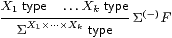
|
but with the normal rules for λ-abstraction and application,
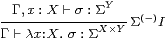
|
together with the usual α, β and η rules Remark B 9.1, ΣY× Z=(ΣZ)Y.
The turnstile (⊢) signifies a sequent presentation in which there are all of the familiar structural rules: identity, weakening, exchange, contraction and cut.
Remark 2.2 As this is a fragment of the simply typed λ-calculus,
it strongly normalises.
We shall take a denotational view of the calculus,
in which the β- and η-rules are
equations between different notations for the same value,
and are applicable at any depth within a λ-expression.
(This is in contrast to the way in which λ-calculi are made to
agree with the execution of programming languages, by restricting the
applicability of the β-rule [Plo75].
Besides defining call by name and call by value
reduction strategies, this paper used continuations to interpret one
dually within the other.)
Notation 2.3 We take account of the restriction on type-formation
by adopting a convention for variable names:
lower case Greek letters and capital italics
denote terms whose type is (a retract of) some ΣX.
These are the terms that can be the bodies of λ-abstractions.
Since they are also the terms to which the lattice operations and ∃
below may be applied, we call them logical terms.
Lower case italic letters denote terms of arbitrary type.
As we have already seen, towers of Σs like ΣΣX tend to arise in this subject. We shall often write Σ2 X, and more generally Σn X, for these. (Fortunately, we do not often use finite discrete types, but when we do we write them in bold: 0, 1, 2, 3.) Increasingly exotic alphabets will be used for terms of these types, including
| a,b,x,y:X φ,ψ:ΣX F,G:ΣΣX F,G:Σ3 X. |
Remark 2.4
In order to model general topology (Section 5)
we must add the lattice operations ⊤, ⊥, ∧ and ∨,
with axioms to say that Σ is a distributive lattice.
In fact, we need a bit more than this.
The Euclidean principle,
| φ:Σ, F:ΣΣ ⊢ φ∧ F(φ) ⇔ φ∧ F(⊤), |
captures the extensional way in which ΣX is a set of subsets [C]. It will be used for computational reasons in Proposition 10.6, and Remark 4.11 explains why this is necessary.
Remark 2.5
We shall also consider the type ℕ of natural numbers,
with primitive recursion at all types, in
Sections 9–10
(where the lattice structure is also needed).
Terms of this type are, of course, called numerical.
Note that ℕ is a discrete set, not a domain with ⊥.
Strong normalisation is now lost.
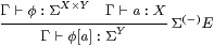
The notation that we use for primitive recursion at type X is
|
where Γ and m:ℕ are static and dynamic parameters, and u denotes the “recursive call”. The β-rules are
| rec(0, z, λ m u.s)=z rec(n+1,z,λ m u.s)=s(n,rec(n, z, λ m u.s)). |
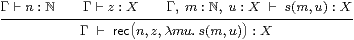
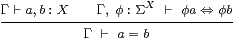
Uniqueness of the rec term is enforced by the rule
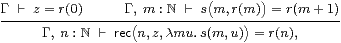
|
whose ingredients are exactly the base case and induction step in a traditional proof by induction. [In fact we need to allow equational hypotheses in the context Γ, see Remark E 2.7.]
Countable joins in ΣΓ may be seen logically in terms of the existential quantifier
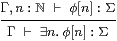
|
for which distributivity is known as the Frobenius law.
Remark 2.6 For both topology and recursion,
a further axiom (called the Scott principle in [Tay91])
is also needed to force all maps to preserve directed joins:
| Γ, F:Σ2ℕ ⊢ F(λ n.⊤) ⇔ ∃ n.F(λ m.m< n). |
For any Γ⊢ G:ΣX→ΣX, let Γ ⊢ Y G = ∃ n.rec (n,λ x.⊥, λ m φ.Gφ) :ΣX and
| Γ, x:X ⊢ F = λφ.G(∃ n.φ n∧ rec (n,λ x.⊥, λ m φ.Gφ))x. |
Then F(λ n.⊤) ⇔ G(Y G)x and ∃ n.F(λ m.m< n) ⇔ Y G x, so Y G is a fixed point of G, indeed the least one. However, this axiom is not needed in this paper, or indeed until we get rather a long way into the abstract Stone duality programme [F][G].
Remark 2.7 We shall want to pass back and forth
between the restricted λ-calculus and the corresponding
category C. The technique for doing this fluently is a major theme
of [Tay99]; see Sections 4.3 and 4.7 in particular.
When a sequent presentation such as ours has all of the usual structural rules (in particular weakening and contraction), there is a category with products
We shall not need the notation ↑ x in this paper, but we shall re-use the . for a different purpose in Section 6. (There we also introduce a category HC that does not have products, but, unlike other authors, we shy away from using a syntactic calculus to work in it, because such a calculus would have to specify an order of evaluation.)
Proposition 2.8 The category C so described is
the free category with finite products and an exponentiating object
Σ, together with the additional lattice and recursive structure
according to the context of the discussion.
Proof The mediating functor ⟦−⟧:C→D from this syntactic category C to another (“semantic”) category D equipped with the relevant structure is defined by structural recursion. ▫
The exponentiating object Σ immediately induces certain structure in the category.
Lemma 2.9 Σ(−) is a contravariant functor.
In particular, for f:X→ Y, ψ:ΣY and F:Σ2 X, we have
| Σf(ψ)=λ x.ψ[f x] and Σ2 f(F)=λ ψ.F(λ x.ψ[f x]). |
Proof You can check that Σid=id and Σf;g=Σg;Σf. ▫
In general topology and locale theory it is customary to write f*ψ⊂ X for the inverse image of ψ⊂ Y under f, but we use Σfψ instead for this, considered as a λ-term, saving f* for the meta-operation of substitution (in Lemmas 8.7 and 9.2).
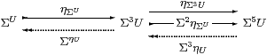
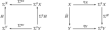
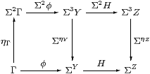
Now we can describe the all-important neighbourhood-family ηX(x) (Remark 1.4) in purely categorical terms. As observed in [Tay99, Remark 7.2.4(c)], it is most unfortunate that the letter η has well established meanings for two different parts of the anatomy of an adjunction.
Lemma 2.10 The family of maps ηX:X→ΣΣX,
defined by x↦(λ φ.φ x),
is natural and satisfies ηΣX;ΣηX=id
(which we call the unit equation).
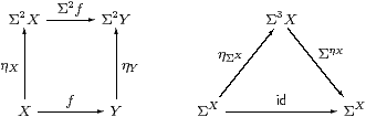
Proof As this Lemma is used extremely frequently, we spell out its proof in the λ-calculus in detail. Using the formulae that we have just given,
| Σ2 f(ηX x)= λψ.(λφ.φ x)(λ x′.ψ(f x′))= λψ.(λ x′.ψ(f x′))(x)=λ ψ.ψ(f x)=ηY(f x). |
Also, ΣηX(F)=λ x.F(ηX x)=λ x.F(λ φ.φ x) for F:Σ3(X), so
| ΣηX(ηΣ Xφ) =λ x.(λ F.Fφ)(λφ′.φ′ x)= λ x.(λ φ′.φ′ x)(φ) =λ x. φ x = φ. ▫ |
Proposition 2.11
The contravariant functor Σ(−)
is symmetrically adjoint to itself on the right,
the unit and counit both being η.
The natural bijection

|
defined by P=ηΓ;ΣH and H=ηX;ΣP is called double exponential transposition.
Proof The triangular identities are both ηΣX;ΣηX=id. ▫
Remark 2.12
The task for the next three sections is to characterise,
in terms of category theory, lambda calculus and lattice theory,
those P:ΣΣX that (should) arise as ηX(a)
for some a:X.
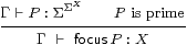
The actual condition will be stated in Corollary 4.12, but, whatever it is, suppose that the morphism or term
| P:Γ→ΣΣX or Γ⊢ P:ΣΣX |
does satisfy it. Then the intuitions of the previous section suggest that we have defined a new value, which we shall call
| Γ⊢focusP:X, |
such that the result of the observation φ:ΣX is
| Γ ⊢ φ(focusP) ⇔ Pφ : Σ. |
In particular, when P≡ηX(a) we recover a=focusP and φ a ⇔ Pφ. These are the β- and η-rules for a new constructor focus that we shall add to our λ-calculus in Section 8.
Remark 2.13 In the traditional terminology of point-set topology,
a completely coprime filter converges to its limit point,
but the word “limit” is now so well established with a completely different
meaning in category theory that we need a new word.
Peter Selinger [Sel01] has used the word “focus” for a category that is essentially our SC. The two uses of this word may be understood as singular and collective respectively: Selinger’s focal subcategory consists of the legitimate results of our focus operator.
We now turn from the type X of values to the corresponding algebra ΣX of observations, in order to characterise the homomorphisms ΣY→ΣX that correspond to functions X→ Y, and also which terms P:ΣΣX correspond to virtual values in X.
Notation 3.1 The adjunction in Proposition 2.11
gives rise to a strong monad with
satisfying six equations. Eugenio Moggi [Mog91] demonstrated how strong monads can be seen as notions of computation, giving a (“let ”) calculus in which µ is used to interpret composition and σ to substitute for parameters. Constructions similar to ours can be performed in this generality.
However, rather than develop an abstract theory of monads, our purpose is to demonstrate the relevance of one particular monad and show how it accounts for the intuitions in Section 1. The associativity law for µ involves Σ6 X, but we certainly don’t want to compute with such λ-terms unless it is absolutely necessary! In fact we can largely avoid using σ and µ in this work.
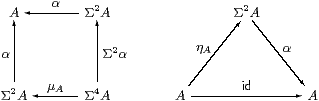
Definition 3.2
An Eilenberg–Moore algebra for the monad is an object A of C
together with a morphism α:Σ2 A→ A such that
ηA;α=idA and µA;α=Σ2 α;α.
Lemma 3.3
For any object X, (ΣX,ΣηX) is an algebra.
Proof The equations are just those in Lemma 2.10, although the one involving µ is Σ(−) applied to the naturality equation for η with respect to ηX. ▫
These are the only algebras that will be used in this paper, but [B]shows how general algebras may be regarded as the topologies on subspaces that are defined by an axiom of comprehension. In other words, all algebras are of this form, but with a generalised definition of the type X.
Definition 3.4 We shall show that the following are equivalent
(when A=ΣX etc.):
We must be careful with the notation JX, as it is ambiguous which way round the product is in the exponent.
Proposition 3.5
If H is a homomorphism or central, and invertible in C,
then its inverse is also a homomorphism or central, respectively. ▫
Lemma 3.6 For any map f:X→ Y in C,
the map Σf:ΣY→ΣX is both a homomorphism and central.
Proof It is a homomorphism by naturality of η, and central by naturality of J(−), with respect to f. ▫
Lemma 3.7
Every homomorphism H:ΣY→ΣX is central.
Proof The front and back faces commute since H is a homomorphism. The left, bottom and top faces commute by naturality of J(−) with respect to ΣH, ηX and ηY. Using the split epi, the right face commutes, but this expresses centrality. ▫
Remark 3.8
To obtain the converse, we ought first to understand how monads
provide a “higher order” account of infinitary algebraic theories
[Lin69].
The infinitary theory corresponding to our monad
has an operation-symbol J of arity U for each morphism
J:ΣU→Σ
(for example, the additional lattice structure consists of morphisms
∧:Σ2→Σ and ⋁:Σℕ→Σ).
Then the centrality square is the familiar rule for
a homomorphism H to commute with the symbol J.
More generally, H commutes with J:ΣU→ΣV iff it is a homomorphism parametrically with respect to a V-indexed family of U-ary operation-symbols. (So, for example, a map J:Σ3→Σ2 denotes a pair of ternary operations.) The next two results are examples of this idea, and we apply it to the lattice structure in the topological interpretation in Proposition 5.5.
Lemma 3.9
H:ΣY→ΣX is a homomorphism with respect to
all constants σ∈Σ,
Proof J=∼id:1→ΣΣ denotes a Σ-indexed family of constants, for which the centrality square is as shown. ▫
The following proof is based on the idea that each r∈ T B corresponds to an operation-symbol of arity B that acts on A as rA:AB→ A by f↦ α(T f r). The rectangle says that K is a homomorphism for this operation-symbol, but it does so for all r∈ T B simultaneously by using the exponential (−)T B.
Thielecke [Thi97a, Lemma 5.2.5] proves this result using his CPS λ-calculus, whilst Selinger [Sel01, Lemma 2.10] gives another categorical proof. They do so with surprisingly little comment, given that it is the Completeness Theorem corresponding to the easy Soundness Lemma 3.7.
Theorem 3.10 All central maps are homomorphisms.
Proof Let H:B=ΣY→ A=ΣX. Writing T for both the functor ΣΣ(−) and its effect on internal hom-sets, consider the rectangle
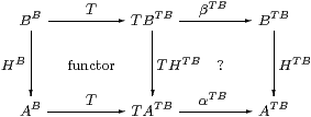
in which the left-hand square says that T preserves composition and the right-hand square that H is an Eilenberg–Moore homomorphism. To deduce the latter, it suffices to show that the rectangle commutes at id∈ BB (which T takes to id∈ TBTB).
Re-expanding, the map along the bottom is ΣX× B→ΣΣ2 X×Σ2 B→ ΣX×Σ2 B by
| θ↦λ F G.G(λ b.F(θ b)) ↦λ x G.G(λ b.ηX x (θ b)) =λ x G.G(λ b.θ b x), |
which is ηΣBX, and similarly the top map is ηΣBY. Thus the rectangle says that H:ΣY→ΣX is central with respect to ηΣB, which was the hypothesis. ▫
[[Proof: Given θ∈ΣX× B, θ:B→ΣX by b↦λ x.θ(x,b), so Σ2θ:Σ2A→Σ3Y by G↦λ F.G(λ b.F(λ x.θ(x,b))). Hence the bottom map takes θ to λ F G.G(λ b.F(λ x.θ(x,b))) and then to λ x G.G(λ b.(λψ.ψ x)(λ x.θ(x,b))) =λ x G.G(λ b.θ(x,b)).]]
Notation 3.11 We write Alg (or sometimes AlgC)
for the category of Eilenberg–Moore algebras and homomorphisms.
Lemma 3.12
For any object X,
(ΣΣX,µX) is the free algebra on X.
In particular,
(Σ, Ση1) is the initial algebra. ▫
Definition 3.13 The full subcategory of Alg consisting
of free algebras is known as the Kleisli category for the monad.
As ΣΣX is free on X, the name of this object in the traditional presentation of the Kleisli category is abbreviated to X, and the homomorphism X→K Y (i.e. ΣΣX→ΣΣY) is named by the ordinary map f:X→ΣΣY. This presentation is complicated by the fact that the identity on X is named by ηX and the composite of f:X→K Y and g:Y→K Z by f;Σ2 g;µZ.
Using the double exponential transpose (Proposition 2.11), this homomorphism is more simply written as an arbitrary map F:ΣY→ΣX, with the usual identity and composition.
The (opposites of the) categories composed of morphisms F:ΣY→ΣX, in the cases where F is an arbitrary C-map (as for the Kleisli category), or required to be a homomorphism, will be developed in Section 6.
Our new notion of sobriety, expressed in terms of the λ-calculus rather than lattice theory, is a weaker form of the fundamental idea of the abstract Stone duality programme.
Definition 4.1
When the category C of types of values is dual to
its category Alg of algebras of observations,
we say that (C,Σ) is monadic.
More precisely, the comparison functor Cop→Alg
defined by Lemmas 3.3 and 3.6,
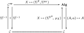
(which commutes both with the left adjoints and with the right adjoints) is to be an equivalence of categories, i.e. full, faithful and essentially surjective.
Remark 4.2
It is possible to characterise several weaker conditions than
categorical equivalence, both in terms of properties of the objects of C,
and using generalised “mono” requirements on ηX.
In particular,
the functor Cop→A is faithful iff all objects are “ T0”
(cf. Remark 1.13),
and also reflects invertibility iff they are replete
[Hyl91, Tay91].
Another way to say this is that each ηX is mono or extremal mono,
and a third is that Σ is a weak or strong cogenerator.
For example, ℕ with primitive recursion is T0 so long as the calculus is consistent, but repleteness and sobriety are equivalent to general recursion [for decidable predicates] (Sections 9–10).
In this paper we are interested in the situation where the functor is full and faithful, i.e. that all homomorphisms are given uniquely by Lemma 3.6. We shall show that the corresponding property of the objects is sobriety, and that of ηX is that it be the equaliser of a certain diagram.
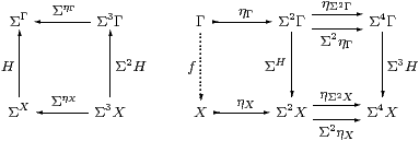
Lemma 4.3
Let (A,α) be an algebra, Γ any object
and H:A→ΣΓ any map in C.
Then H is a homomorphism iff its double exponential transpose
P:Γ→ΣA (Proposition 2.11) has equal composites
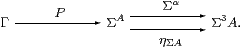
Proof We have H=ηA;ΣP and P=ηΓ;ΣH. [⇒] P;Σα=ηΓ;ΣH;Σα=ηΓ;Σ2ηΓ;Σ3 H =ηΓ;ηΣ2 Γ;Σ3 H=ηΓ;ΣH;ηΣ A =P;ηΣ A. [⇐] α;H=α;ηA;ΣP=ηΣ2 A;Σ2α;ΣP =ηΣ2 A;ΣηΣ A;ΣP=ΣP =Σ2ηA;ΣηΣ A;ΣP =Σ2ηA;Σ3 P;ΣηΓ=Σ2 H;ΣηΓ. ▫
Corollary 4.4
The (global) elements of the equaliser are the those functions
A→Σ that are homomorphisms. ▫
Definition 4.5 Such a map P is called prime.
(We strike through the history of uses of this word, such as in
Definition 1.7 and Corollary 5.8.
In particular, although the case X=ℕ will turn out to be
the most important one, we are not just talking about
the numbers 2, 3, 5, 7, 11, ...!)
As we always have A=ΣX in this paper,
we usually write P as a term Γ⊢ P:ΣΣX.
Lemma 4.6
In Lemma 4.3, ηX is the prime
corresponding to the homomorphism id:ΣX→ΣX.
If P:Γ→ΣA is prime and J:B→ A a homomorphism
then P;ΣJ is also prime.
In particular, composition with Σ2 f preserves primes.
▫
Definition 4.7
We say that an object X∈obC is sober if the diagram
is an equaliser in C, or, equivalently, that the naturality square
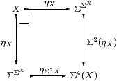
for η with respect to ηX is a pullback.
Remark 4.8 We have only said that
the existing objects can be expressed as equalisers,
not that general equalisers can be formed.
In fact, this equaliser is of the special form described below,
which Jon Beck exploited to characterise monadic adjunctions
[Mac71, Section VI 7], [BW85, Section 3.3],
[Tay99, Section 7.5].
The category will be extended to include such equalisers,
so we recover a space pts(A,α) from any algebra,
in [B].
Notice the double role of Σ here, as both a space and an algebra. Peter Johnstone has given an account of numerous well known dualities [Joh82, Section VI 4] based the idea that Σ is a schizophrenic object. (This word was first used by Harold Simmons, in a draft of [Sim82], but removed from the published version.)
Moggi [Mog88] called sobriety the equalizing requirement, but did not make essential use of it in the development of his computational monads.
Applegate and Tierney [Eck69, p175] and Barr and Wells [BW85, Theorem 3.9.9] attribute these results for general monads to Jon Beck. See also [KP93] for a deeper study of this situation.
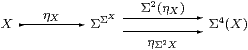
Proposition 4.9 Any power, ΣU, is sober.
Proof This is a split equaliser: the dotted maps satisfy
|
by Lemma 2.10, the equations on the right being naturality of η with respect to ΣηU and ηΣU. Hence if P:Γ→Σ3 U has equal composites then P=P;ΣηU;ηΣU, and the mediator is P;ΣηU. ▫
Theorem 4.10
The functor Σ(−):Cop→Alg given in Definition 4.1
is full and faithful iff all objects are sober.
Proof [⇒] We use P:Γ→Σ2 X to test the equaliser. By Lemma 4.3, its double transpose H:ΣX→ΣΓ is a homomorphism, so by hypothesis H=Σf=ηΣX;ΣP for some unique f:Γ→ X, and this mediates to the equaliser.
[⇐] Let H:ΣX→ΣΓ be a homomorphism, so the diagram on the left above commutes, as do the parallel squares on the right, the lower one by naturality of Ση with respect to H. Since X is the equaliser, there is a unique mediator f:Γ→ X, and we then have H=ηΣX;ΣP=ηΣX;ΣηX;Σf=Σf. ▫
Remark 4.11
Translating Definition 1 into the λ-calculus,
the property of being a homomorphism H:ΣX→ΣU
can be expressed in a finitary way
as an equation between λ-expressions,
| F:Σ3 X⊢(λ u.F(λφ.Hφ u)) = H(λ x.F(λφ.φ x)), |
the two sides of which differ only in the position of H.
The double exponential transpose P of H is obtained in the λ-calculus simply by switching the arguments φ and u (cf. Remark 1.11). Hence ⊢ P:U→ΣΣX is prime iff
| u:U, F:Σ3 X ⊢ F(P u) = P u(λ x.F(λφ.φ x)). |
Replacing the argument u of P by a context Γ of free variables, Γ⊢ P:ΣΣX is prime iff
| Γ, F:Σ3 X ⊢ F P ⇔ P(λ x.F(λφ.φ x)) |
or F P ⇔ P(ηX;F). This is the equation in Lemma 4.3, with A=ΣX, applied to F.
[In the context of the additional lattice structure, including Scott continuity, P is prime iff it preserves ⊤, ⊥, ∧ and ∨ Theorem G 10.2.]
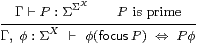
Corollary 4.12 The type X is sober iff
for every prime Γ⊢ P:Σ2 X
there is a unique term Γ⊢focusP:X such that
| Γ, φ:ΣX ⊢ φ(focusP) ⇔ Pφ. |
Hence the side-condition on the introduction rule for focusP in Remark 2.12 is that P be prime. Indeed, since φ↦φ x is itself a homomorphism (for fixed x), this equation is only meaningful in a denotational reading of the calculus when P is prime. (On the other hand Thielecke’s force operation has this as a β-rule, with no side condition, but specifies a particular order of evaluation.) ▫
Remark 4.13 So far, we have used none of the special structure on Σ in
Remarks 2.4ff. We have merely used the restricted
λ-calculus to discuss what it means for the other objects of
the category to be sober with respect to it.
In Sections 6–8
we shall show how to enforce this kind of sobriety on them.
If P=ηX(x) then the right hand side of the primality equation easily reduces to the left. Otherwise, since F is a variable, the left hand side is head-normal, and so cannot be reduced without using an axiom such as the Euclidean principle (Remark 2.4), as we shall do in Proposition 10.6.
The introduction of subspaces [B][E]also extends the applicability of the equation, by allowing it to be proved under hypotheses, whilst using the continuity axiom (Remark 2.6) it is sufficient to verify that P or H preserves the lattice connectives. In other words, the mathematical investigations to follow serve to show that the required denotational results are correctly obtained by programming with computational effects.
Remark 4.14 In his work on continuations, Hayo Thielecke uses R
for our Σ and interprets it as the answer type.
This is the type of a sub-program that is called like a function,
but, since it passes control by calling another continuation,
never returns “normally” — so the type of the answer is irrelevant.
Thielecke stresses that R
therefore has no particular properties or structure of its own.
In the next section, we shall show that the Sierpiński space in topology behaves categorically in the way that we have discussed, but it does carry additional lattice-theoretic structure.
Even though a function or procedure of type void never returns a “numerical” result — and may never return at all — it does have the undisguisable behaviour of termination or non-termination. Indeed, we argued in Remark 1.2 that termination is the ultimate desideratum, and that therefore the type of observations should also carry the lattice structure. Proposition 10.6, which I feel does impact rather directly on computation, makes use of both this structure and the Euclidean principle.
[The referee pointed out that there are, in practice, other computational effects besides non-termination, such as input–output.]
Thielecke’s point of view is supported by the fact that the class of objects that are deemed sober depends rather weakly on the choice of object Σ: in classical domain theory, any non-trivial Scott domain would yield the same class.
Remark 4.15 Although it belongs in general topology, sobriety was first
used by the Grothendieck school in algebraic geometry
[AGV64, IV 4.2.1]
[GD71, 0.2.1.1] [Hak72, II 2.4].
They exploited sheaf theory, in particular the functoriality of
constructions with respect to the lattice of open subsets, the points
being secondary.
An algebraic variety (the set of solutions of a system of polynomial equations) is closed in the Euclidean topology, but there is a coarser Zariski topology in which they are defined to be closed. When the polynomials do not factorise, the closed set is not the union of non-trivial closed subsets, and is said to be irreducible. A space is sober (classically) iff every irreducible closed set is the closure of a unique point, known in geometry as the generic point of the variety. Such generic points, which do not exist in the classical Euclidean topology, had long been a feature of geometrical reasoning, in particular in the work of Veronese (c. 1900), but it was Grothendieck who made their use rigorous.
In this section we show how the abstract categorical and symbolic structures that we have introduced are equivalent to the traditional notions in general topology that we mentioned in Section 1. In fact, all that we need to do is to re-interpret lattice-theoretic work that was done in the 1970s. On this occasion our treatment will be entirely classical, making full use of the axiom of choice and excluded middle; for a more careful intuitionistic account see [B][C][G][H].
If you are not familiar with locally compact topological spaces, you may consider instead your favourite category of algebraic (or continuous) predomains, which are all sober. The discrete space ℕ is also needed, besides domains with ⊥. The results of this section are only used as motivation, so you can in fact omit it altogether.
Alternatively, the construction may be performed with arbitrary dcpos, although it adds extra points to those that are not sober. Peter Johnstone gave an example of such a non-sober dcpo [Joh82, Exercise II 1.9], as part of the philosophical argument against point-set topology. We shall not need this, as the localic view is already deeply embedded in our approach. In fact, when we construct new spaces in [B], they will be carved out as subspaces of lattices (cf. [Sco72]) not glued together from points.
Remark 5.1 The classical Sierpiński space Σ has two points:
⊤ is open and ⊥ is closed. So altogether there are
three open sets: ∅, {⊤} and Σ.
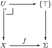
This space has the (universal) property that, for any open subset U of any space X, there is a unique continuous function f:X→Σ such that the inverse image f*⊤ is U. Indeed, f takes the points of U to ⊤, and those of its closed complement to ⊥.
This is the same as the defining property of the subobject classifier Ω in a topos, except that there U⊂ X can be any subobject. We shall discuss sobriety for sets, discrete spaces and objects of a topos in Section 9.
Hence open subsets of X correspond bijectively to maps X→Σ, and so to points of the exponential ΣX. In other words, the space ΣX is the lattice of open subsets of X, equipped with some topology.
Remark 5.2 Finite intersections and arbitrary unions of open subsets
give rise to internal lattice structure on Σ, written
∧:Σ×Σ→Σ and ⋁:ΣU→Σ.
Besides the infinite distributive law,
conjunction also satisfies the Euclidean principle (Remark 2.4).
Whilst this is vacuous classically, it and its lattice dual
(which says that ⊥ classifies closed subsets)
capture remarkably much of the flavour of locale theory
[C][D],
before we need to invoke the continuity axiom (Remark 2.6),
though of course that is also valid in topology.
Remark 5.3 To determine the topology on the space ΣX,
consider the map ev:ΣX× X→Σ.
For this to be continuous,
Ralph Fox showed that the space X must be locally compact,
and ΣX must have the compact–open topology [Fox45],
which is the same as the Scott topology when we only consider Σ
and not more general target spaces.
The categorical analysis is due to John Isbell [Isb75].
Local compactness is a very familiar notion for Hausdorff spaces, but there are messy subtleties to its definition for non-Hausdorff spaces [HM81]. However, so long as we only consider spaces that are sober in the standard topological sense, things are not too difficult:
For any point x and open subset x∈ U⊂ X, there must be a compact subset K and another open subset V with x∈ V⊂ K⊂ U. The “open rectangle” around (U,x)∈ev−1{⊤}⊂ΣX× X that we need for continuity of ev is then
{W∈ΣX ∣ K⊂ W}× V ⊂ ΣX× X.
In the jargon, X has a base of compact neighbourhoods, cf. Bourbaki’s usage in Remark 1.8.
All of this is much prettier in terms of the open sets: the topology ΣX is a distributive continuous lattice, equipped with the Scott topology. Such a lattice is of course a frame, and the corresponding locale is called locally compact. Assuming the axiom of choice, the category LKLoc of locally compact locales is equivalent to the category LKSp of locally compact sober spaces [Joh82, Section VII 4.5].
Remark 5.4 Since ΣX carries the Scott topology,
a continuous function ΣY→ΣX
is a function between open set lattices that preserves directed unions.
Such a function is called Scott-continuous.
In particular, it preserves the order that is induced by the lattice structure
[Sco72].
Besides frame homomorphisms themselves, functions like this between frames do arise in general topology. For example, a space K is compact iff Σ!K:Σ→ΣK has a Scott-continuous right adjoint, ⋀:ΣK→Σ. Unfortunately, monotone functions between frames that need not preserve directed joins are also used in general topology, and these present the main difficulty that abstract Stone duality faces in re-formulating the subject [D].
Proposition 5.5
Let H:ΣX→ΣU be a Scott-continuous function
between the topologies of locally compact spaces.
If H is central (Definition 2) then it
preserves finite meets and arbitrary joins.
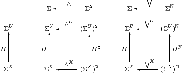
Proof Lemma 3.9 dealt with the constants (⊤ and ⊥), so consider J=∧:Σ2→Σ and ⋁:Σℕ→Σ. ▫
Remark 5.6 We also have ⋁:ΣU→Σ for any space U,
together with the associated distributive law.
In the case of U=ℕ, we write ∃ for ⋁,
and distributivity is known as the Frobenius law,
| ψ∧∃ n.φ(n) = ∃ n.ψ∧φ(n). |
We have ⋀:ΣK→Σ only when K is compact; in particular, it would be ∀ for K=ℕ, but (ℕ is not a compact space and) ∀ℕ is not computable (cf. Definition 1.3). Indeed, in a constructive setting, ⋁:ΣU→Σ only exists for certain spaces U, which are called overt (Section C 8). Overtness is analogous to recursive enumerability, cf. Remark 9.12 and Lemma 10.2.
We are now ready to show how our new λ-calculus formulation in Sections 3–4 captures the hitherto lattice-theoretic ideas of continuous functions and sober spaces. A proof entirely within abstract Stone duality (including the continuity axiom) that preserving the lattice operations suffices will be given in Theorem G 10.2.
Theorem 5.7
Let U and X be locally compact sober spaces and
H:ΣX→ΣU a Scott-continuous function between their topologies.
Then the following are equivalent:
[[[e=f] 4.11; [e⇒d] 3.7; [d⇒e] 3.10; [d⇒c] 5.5; [c⇒b] easy; [b⇒c] by Scott continuity; [a⇒d,e] 3.6.]]
Proof [[d⇒c]] We have just shown that central maps are frame homomorphisms.
[[c⇒a]] Since X is sober in the topological sense, all frame homomorphisms ΣX→ΣU are of the form Σf for some unique f:U→ X (we take this as the topological definition of sobriety). But all Σf are Eilenberg–Moore homomorphisms. ▫
Corollary 5.8 The following are equivalent for
P:1→ΣΣX:
Similarly, for a continuous function P:U→ΣΣX, the same equivalent conditions hold for P(u) for each point u∈ U. ▫
Remark 5.9 Our primes are therefore what Johnstone calls
the “points” of the locale ΣX,
so sobriety for LKSp in our sense agrees with his
[Joh82, Section II 1.6].
As a topological space, the equaliser is the set U of primes,
equipped with the sparsest locally compact topology
such that U→Σ2 X is continuous,
and the hom-frame C(X,Σ) provides this topology.
Remark 5.10
We have a theorem in the straightforward sense for LKSp
that says that, given a Scott-continuous map H:ΣX→ΣU
between the open-set lattices of given locally compact spaces,
H is a homomorphism of frames if and only if it is a homomorphism
in the sense of our monad.
By contrast, the notions of sobriety expressed in terms of lattice theory and the λ-calculus agree only in intuition. We are only able to bring these two mathematical systems together in a setting where topological sobriety has already been assumed. If you are skeptical of the mathematical status of the argument, consider the analogous question in the relationship between locales and Bourbakian spaces: at what point in the axiomatisation of locales do we make the assumption that renders them all sober? Even then, these two categories only agree on their products on the same subcategory as ours, namely locally compact spaces. In summary, the concordance of several approaches (along with [G], and models of synthetic domain theory [Tay91]) makes us confident that the notion of locally compact space is a good one, but not so sure how it ought to be generalised.
Remark 5.11 The types of the restricted λ-calculus,
even with the additional lattice and recursive structure,
form a very impoverished category of spaces.
Identifying them with their interpretations in LKSp,
they amount merely to (some of) the algebraic lattices
that Dana Scott used in the earliest versions of his denotational semantics
[Sco76],
and include no spaces at all (apart from 1 and ℕ)
that would be recognisable to a geometric topologist.
The monadic property populates the category of spaces with subspaces of the types of the restricted λ-calculus. We show how to do this in terms of both abstract category theory and as an extension of the λ-calculus similar to the axiom of comprehension in [B], which also proves the next result intuitionistically for locales.
Although we only intended to consider sobriety and not monadicity in this paper, we actually already have enough tools to characterise the algebras for the monad classically in lattice-theoretic terms. Further proofs appear in [B][G][H].
Proof As all of the spaces are sober, the functor in Definition 4.1 is full and faithful. It remains to show that every Eilenberg–Moore algebra (A,α) is of the form (ΣX,ΣηX) for some locally compact space X. But, as A is a retract of a power of Σ, it must be a continuous lattice equipped with the Scott topology, and must in fact also be distributive, so A≅ΣX for some locally compact sober space X.
However, we still need to show that the Eilenberg–Moore structure α:Σ2 A→ A is uniquely determined by the order on A, and is therefore ΣηX as in Lemma 3.3.
For this, we must determine α F for each element F∈Σ2 A; such F defines a Scott-open subset of the lattice ΣA. It can be expressed as a union of Scott-open filters in this lattice, i.e. these filters form a base for the Scott topology [Joh82, Lemma VII 2.5] [GHK++80, Section I.3]. Since α must preserve unions, it suffices to define α F when F is a Scott-open filter.
Now each Scott-open filter F itself corresponds to compact saturated subspace K⊂ A [HM81, Theorem 2.16], cf. Remark 1.10. For a lattice A with its Scott topology, a “saturated” subspace is simply an upper set. Since α must be monotone and satisfy ηA;α=idA, we have α(F)≤ a for all a∈ K. For the same reason, if b∈ A satisfies ∀ a. a∈ K⇒ b≤ a then b≤α(K). Hence α(F)=⋀ K∈ A. Thus the effect of α on all elements of Σ2 A has been fixed, as a join of meets. ▫
Setting aside the discussion of more general spaces, what we learn from this is that, when all objects are sober, there are “second class” maps between objects. We shall see in the next section that this phenomenon arises for abstract reasons, and that the potential confusion over (Scott-) “continuous maps between frames” is not an accident.
Now we turn from the analysis to the synthesis of categories that have all objects sober. So our primary interest shifts from locales to the restricted λ-calculus in Remark 2.1.
Since we handle continuous functions f:X→ Y in terms of the corresponding inverse image maps Σf, it is natural to work in a category in which there are both “first class” maps f:X→ Y (given concretely by homomorphisms Σf:ΣY→ΣX) and “second class” maps F:X−× Y that are specified by any F:ΣY→ΣX.
These second class maps — ordinary functions rather than homomorphisms between algebras — are just what is needed to talk about U-split (co)equalisers as in Beck’s theorem (cf. Proposition 4.9 and [B]). Even in more traditional subjects such as group and ring theory, we do indeed sometimes need to talk about functions between algebras that are not necessarily homomorphisms.
The practical reason for according these maps a public definition is that the product functor is defined for them (Proposition 6.5), and this will be crucial for constructing the product of formal Σ-split subspaces in [B]. After I had hesitated on this point myself, it was seeing the work of Hayo Thielecke [Thi97b] and Carsten Führmann [Füh99] on continuations that persuaded me that this is the best technical setting, and this section essentially describes their construction.
As to the first class maps, the whole point of sobriety is that they consist not only of f:X→ Y in C, but other maps suitably defined in terms of the topology.
Definition 6.1
The categories HC and SC both have the same objects as C, but
Thielecke and Führmann call these thunkable morphisms, since they write thunkX for ηX considered as an HC-map. It follows immediately (given Theorem 3.10) that ηX:X→ΣΣX is natural in SC but not HC.
Identity and composition are inherited in the obvious way from C, though contravariantly, which is why we need the F notation (which [Sel01, Section 2.9] also uses).
Remark 6.2 By Lemma 3.6, for f:X→ Y in C,
the map H=Σf:ΣY→ΣX is a homomorphism,
so H:X→ Y is in SC.
We shall just write this as f:X→ Y instead of Σf:X→ Y,
but beware that, in general,
different C-maps can become equal SC-maps with the same names.
By Remark 4.2, this functor C→SC is faithful iff every object of C is T0, and it also reflects invertibility if every object is replete. Theorem 4.10 said that it is also full iff every object of C is sober; as SC and C have the same objects, they are then isomorphic categories.
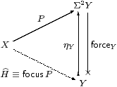
There are, of course, many more morphisms in HC than in C, but one (family) in particular generates the rest. We shall see that the new second class morphism force:Σ2 X−× X objectifies the operation P↦focusP that is only defined when P:Σ2 X is prime. Thielecke and Führmann apply their β-rule for force without restriction, producing computational effects, whilst our side-condition on focus gives it its denotational or topological meaning.
Definition 6.3
forceX = ηΣX : ΣΣX −× X
is a natural transformation in the category HC,
and satisfies ηX;forceX=idX or force(thunkx)=x.
Proof This is Lemma 2.10 again. force(−) in HC is ηΣ(−) in C, which is natural (in C) with respect to all maps F:ΣY→ΣX, so force(−) is natural (in HC) with respect to F:X−× Y. The other equation is ηΣX;ΣηX=idX. ▫
Corollary 6.4
The C-map ηX:X→Σ2 X is mono in both HC and SC.
Proof It is split mono in HC, and remains mono in SC because there are fewer pairs of incoming maps to test the definition of mono. ▫
Proposition 6.5 For each object X,
the product X×− in C extends to an endofunctor on HC.
This construction is natural with respect to C-maps
f:X→ Y (so H=Σf).
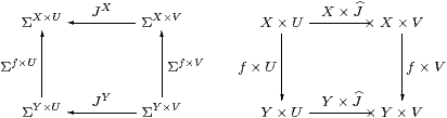
Proof For J:V−× U in HC, i.e. J:ΣU→ΣV in C, we write X× J:X× V−× X× U for the C-map JX:ΣX× U→ΣX× V. This construction preserves identities and composition because it is just the endofunctor (−)X defined on a subcategory of C. It extends the product functor because, in the case of a first class map g:V→ U (so J=Σg:ΣU→ΣV), we have X× J=X×Σg=ΣX× g=X× g, which is a first class map X× V→ X× U.
The construction is natural with respect to f:X→ Y because J(−) is. ▫
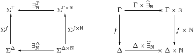
Example 6.6 The existential quantifier ∃ℕΓ in the context Γ
is obtained in this way,
and its Beck–Chevalley condition with respect to the substitution or cut
f:Γ→Δ
Proposition C 8.1 is commutativity of the square
(cf. Proposition 5.5):
Example 6.7
× is not defined as a functor of two variables on HC,
because the squares
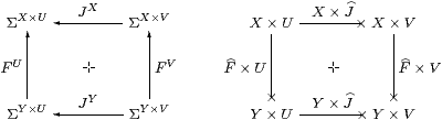
do not necessarily commute (+ [FS90]). For example, take F=J:Σ−×0 where F=J:Σ0=1→ΣΣ is the element ∼id∈ΣΣ; then these two composites give the elements ∼π0,∼π1∈ΣΣ×Σ.
Remark 6.8 × is a premonoidal structure
on HC in the sense of John Power [Pow02],
and a map F makes the square commute for all J
iff F is central (Definition 2).
Thielecke, Führmann and Selinger begin their development from HC
as a premonoidal category, whereas we have constructed it as
an intermediate stage on the journey from C to SC.
Definition 6.9
F:X−× Y is discardable or copyable
respectively if it respects the naturality of
the terminal (or product) projection (!) and the diagonal (Δ).
These terms are due to Hayo Thielecke [Thi97a, Definition 4.2.4], who demonstrated their computational meaning (op. cit., Chapter 6). In particular, non-terminating programs are not discardable, but he gave examples of programs involving control operators that are discardable but not copyable, so both of these properties are needed for a program to be free of control effects such as jumps (Remark 1.5). In fact, these conditions are enough to characterise first class maps in the topological interpretation [F], but not for general computational effects [Füh02]. [See the appendix to [F].]
Lemma 6.10 Δ is natural in SC,
i.e. all first class maps are copyable.
Proof As in Lemma 3.7, we show that the above diagram commutes by making it into a cube together with
which commutes by naturality of Δ in C, as do the side faces of the cube, the other edges being ηX, ηX×ηY, etc. The top and bottom faces commute because H is a homomorphism and by naturality of H(−) and (Σ2 H)(−) with respect to ηX and ηY. The original diagram therefore commutes because ηY×ηY is mono by Corollary 6.4. ▫
Proposition 6.11
SC has finite products and C→SC preserves them.
Proof The terminal object 1 is preserved since Σ is the initial algebra (Lemma 3.12). The product projections and diagonals are inherited from C, so Δ;p0=id=Δ;p1 and Δ;(p0× p1)=id.
Then, for SC-maps a=H:Γ→ X and b=K:Γ→ Y, we obtain <a,b> as Δ;a× b, but we need centrality (Lemma 3.7) to make a× b well defined.
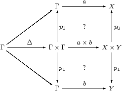
The issue is that the squares commute. In C, the upper one is
using one of the two definitions for H×K=a× b. The left-hand square commutes by Lemma 3.7 because K:ΣY→ΣΓ is discardable (as it is a homomorphism), and the right-hand square by naturality of H(−):ΣX×(−)→ΣΓ×(−) with respect to !:Y→1.
For uniqueness, suppose that f;p0=a and f;p1=b. Then
|
We still have to show that SC has powers of Σ, and that all of its objects are sober. In fact SC freely adjoins sobriety to C.
Lemma 7.1
Still writing Σ(−) for the exponential in C,
SC(X,ΣY)≅ C(X,ΣY),
where the homomorphism H:Σ2 Y→ΣX
corresponds to the map f:X→ΣY by
| H=Σf and f=ηX;ΣH;ΣηY. |
Proof H∈SC(X,ΣY) is by definition a homomorphism H:Σ2 Y→ΣX, whose double exponential transpose P:X→Σ3 Y has equal composites with Σ3 Y⇉Σ5 Y by Lemma 4.3, and so factors as f:X→ΣY through the equaliser by Proposition 4.9. More explicitly,
| ηX;ΣΣf;ΣηY = f;ηΣY;ΣηY = f |
by Lemma 2.10, and
| Σf = ΣΣηY;ΣΣH;ΣηX = ΣΣηY;ΣηΣY;H = H |
since H is a homomorphism. ▫
Proposition 6.11 (and the way in which objects of SC are named) allow us to use the product notation ambiguously in both categories. Relying on that, we can now also justify writing ΣX for powers in either C or SC.
Corollary 7.2 SC has powers of Σ and
C→SC preserves them.
Proof SC(Γ×SC X,Σ) = SC(Γ×CX,Σ) by Proposition 6.11. Then by the Lemma this is C(Γ× X,Σ) ≅ C(Γ,ΣX)≅SC(Γ,ΣX). ▫
Proof AlgSC is defined from SC in the same way as AlgC≡Alg is defined from C (Definition 3.2). Consider the defining square for a homomorphism over SC:
The vertices are retracts of powers of Σ, and Lemma 7.1 extends to such objects. Hence the SC-maps α, β and H might as well just be C-maps, by Lemma 7.1, and the equations hold in SC iff they hold in C. ▫
Proposition 7.4 All objects of SC are sober,
SSC≅SC and HSC≅HC.
Proof The categories all share the same objects, and by Lemma 7.1,
| HSC(X,Y) = SC(ΣY,ΣX) ≅ C(ΣY,ΣX) = HC(X,Y). |
Lemma 7.3 provides the analogous result for SC, namely
| SSC(X,Y) = AlgSC(ΣY,ΣX) ≅ Alg(ΣY,ΣX) = SC(X,Y). |
Then all objects of SC are sober by Theorem 4.10. ▫
By Corollary 4.12, SC therefore has focusP for every prime P. The construction in the previous section shows that this is given by composition with the second class map force.
Proof The correspondence between H and P is double exponential transposition (Proposition 2.11), and H is a homomorphism (i.e. H is in SC) iff P is prime, by Lemma 4.3. In particular, H=idΣX corresponds to P=ηX. When H is a homomorphism we have
| P = ηX;ΣH = ηX;Σ2 |
| = |
| ;ηY, |
or thunk(a), where x:X⊢ a:Y is the term corresponding to H, so
| focusP = focus(thunka) = a. ▫ |
Theorem 7.6 SC is, up to isomorphism,
the universal way of forcing all objects of C to be sober.

Proof Let D be a category with products and an exponentiating object ΣD, and let F:C→D be a functor that preserves this structure. Suppose that all objects of D are sober. Given any homomorphism H:ΣY→ΣX in C, consider its image under the functor in D. This is a homomorphism F H:ΣDF Y→ΣDF X since F commutes with Σ(−) and preserves the Eilenberg–Moore equation. Therefore F H is of the form ΣDg for some unique g:F X→ F Y, since all objects of D are sober. Then g is the effect of F on the given SC-morphism H:X→ Y.
This construction preserves identities and compositions by the usual uniqueness arguments, and similarly if H=Σf with f:X→ Y in C then g=F f. Hence we have a commutative triangle of functors. As the objects X and Y of SC are just objects of C and F(X× Y)≅ F X× F Y on C, products in SC are also preserved, as are powers of Σ. ▫
Remark 7.7 Peter Selinger, for whom (his version of) the computational
category HC is of primary interest,
calls C and SC value categories,
and takes an egalitarian view of them [Sel01, Section 3.5].
However, we have just shown that SC has a universal property,
so it is the sober completion of C,
and such (established) language does make a value-judgement:
we regard SC as better than C,
since it includes denotational values that we have argued ought
to be present.
Be careful, however, to distinguish this sober completion of the category C from the sobrification X of the space (object) X [Joh82, Corollary II 1.7(ii)]. If C has equalisers, X is obtained by forming the equaliser that we used to define sobriety (cf. Remark 4.8). In [B]we shall obtain the space pts(A,α) of points of an arbitrary algebra by forming an equaliser of this kind. These “concrete” constructions on objects are carried out within a single sufficiently expressive category, whereas SC is a new category that is obtained “abstractly” by re-naming features of the old category C.
Remark 7.8 What of the extra structure in Remarks 2.4ff?
The lattice operations ⊤, ⊥, ∧ and ∨, being
morphisms 1→Σ or Σ×Σ→Σ in C,
are carried by the functor C→SC into the new category.
The equations for a distributive lattice still hold,
because any functor preserves equations, and this one also preserves products.
The Euclidean principle remains valid in the new category too,
as ΣΣ is also preserved.
This leaves ℕ, from which preservation of the existential quantifier and
continuity axiom follow easily.
The only issue is in fact the way in which new values are created in SC by the combination of focus and primitive recursion. We leave the reader to add parameters: S:Γ×ℕ× X→ X.
Proposition 7.9 C→SC preserves the natural numbers object,
i.e. ℕ admits primitive recursion in SC.
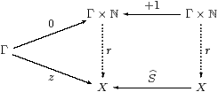
Proof The recursion data consist of z:Γ→ X and a homomorphism S:ΣX→ΣX. So Z≡ z;ηX is prime and has equal composites in the lower triangle below, whilst the parallel squares each commute, by naturality of η.
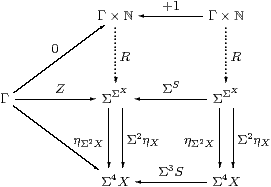
As ℕ has the universal property in C, there are mediators R:Γ×ℕ→Σ2 X and Γ×ℕ→Σ4 X making the whole diagram commute. But, by uniqueness of the second, the composites Γ×ℕ⇉Σ4 X are equal, so R is prime by Lemma 4.3, and focusR:ℕ→ X is the required mediator in SC. ▫
Finally, we note a result that would hold automatically if SC were a cartesian closed category.
Lemma 7.10 The functor SC→Cop preserves such colimits as exist.
Proof The diagram for a colimit in SC is a diagram for a limit in C whose vertices are powers of Σ and whose edges are homomorphisms. If the diagram has a colimit C in SC then it is a cone of homomorphisms in C with vertex ΣC whose limiting property is tested by other cones of homomorphisms from powers of Σ. We have to extend this property to cones from arbitrary objects Γ of C.
Let φ:Γ→ΣY be a typical edge of the cone and H:ΣY→ΣZ an edge of the diagram. Then Σ2φ;ΣηY:Σ2Γ→ΣY is a homomorphism, and is an edge of a cone with vertex Σ2Γ because the diagram above commutes.
Hence there is a mediator Γ→Σ2Γ→ΣC to the limit. It is unique because any other such mediator Γ→ΣC can be lifted to a homomorphism Σ2Γ→ΣC in the same way, and this must agree with the mediator that we have. ▫
Proposition 7.11
The functor X×(−) preserves (distributes over)
such colimits as exist in SC.
Proof The functor X×(−) on SC is (−)X on C, which is defined at powers of Σ and homomorphisms between them. If C is the colimit of a diagram with typical edge H:Z→ Y in SC then the Lemma says that ΣC is the limit of the diagram with typical edge H:ΣY→ΣZ in C. Now (−)X, in so far as it is defined, preserves limits, since it has a left adjoint X×(−) in C. (You may like to draw the diagrams to show this explicitly.) Hence ΣC× X is the limit of the diagram with typical edge HX:ΣX× Y→ΣX× Z in C. Since fewer (co)cones have to be tested, C× X is the colimit of the diagram with typical edge X×H:X× Y→ X× Z in SC. ▫
In this section we show that SC interprets the restricted λ-calculus, together with the new operation focus. For reference, we first repeat the equation in Remark 4.11.
Definition 8.1 Γ⊢ P:ΣΣX is
prime if Γ, F:Σ3 X ⊢
F P ⇔ P(λ x.F(λφ.φ x)).
Definition 8.2 The sober λ-calculus
is the restricted λ-calculus (Definition 2.1)
together with the additional rules
 focusI
|
 focusβ
|
 T0
T0
|
The definition thunka = ηX(a) = λ φ.φ a serves as the elimination rule for focus. Using this, equivalent ways of writing the focusβ and η (T0) rules are
| thunk (focusP)=P and focus (thunkx) = x, |
where P is prime.
Remark 8.3 The restriction of focus to primes
is the crucial difference from Thielecke’s force calculus,
and is the reason why we gave it a new name.
In the focusβ-rule,
how can we tell how much of the surrounding expression
is the predicate φ that is to become the sub-term of P?
For example, for F:ΣΣ,
| does F(φ(focusP)) reduce to F(Pφ) or to P(φ;F) ? |
So long as P is prime, it doesn’t matter, because these terms are equal. In Remark 11.4 we consider briefly what happens if this side-condition is violated.
Proof The double transpose H:ΣX→ΣΓ of P is a homomorphism with respect to the double transpose J:Σ→ΣΓ of F. ▫
The interaction of focus with substitution, i.e. cut elimination, brings no surprises.
Lemma 8.4 If Γ⊢ P:Σ2 X is prime
then so is Δ⊢ (u*P):Σ2 X for any substitution
u:Δ→Γ [Tay99, Section 4.3], and then
| Δ ⊢ u*(focusP) = focus(u*P) :X. |
Proof In the context [Δ, F:Σ3 X], since x, φ and F don’t depend on Γ,
| F(u*P) ≡ u*(F P) = u*(P(λ x.F(λφ.φ x))) ≡ (u*P)(λ x.F(λφ.φ x)), |
so u*P is prime. Then, in the context [Δ, φ:ΣX],
| φ(u*(focusP)) ≡ u*(φ(focusP)) = u*(Pφ) ≡ (u*P)φ = φ(focus(u*P)) |
using the focusβ-rule, whence the substitution equation follows by T0. ▫
Theorem 8.5 SC is a model of the sober λ-calculus.
Proof Since SC has products and powers of Σ (Proposition 6.11 and Corollary 7.2), it is a model of the restricted λ-calculus. Lemma 7.5 provides the interpretation of focusP and (the second form of) its β- and η-rules. ▫
Remark 8.6
Let C and D be the categories corresponding to
the restricted and sober λ-calculi respectively,
as in Remark 2.7.
Since the calculi have the same types, and so contexts,
D has the same objects as C and SC.
We have shown how to interpret focus in SC, and that the equations are valid there. Hence we have the interpretation functor ⟦−⟧:D→SC in the same way as in Proposition 2.8, where ⟦−⟧ acts as the identity on objects (contexts).
Since D interprets focus by definition, all of the objects of D are sober by Corollary 4.12. The universal property of SC (Theorem 7.6) then provides the inverse of the functor ⟦−⟧, making it an isomorphism of categories.
Alternatively, we can show directly that D has the same morphisms as SC, by proving a normalisation result for the sober λ-calculus. Besides being more familiar, this approach demonstrates that we have stated all of the necessary equations in the new calculus. We have already shown that the new calculus is a sound notation for morphisms of the category SC, and it remains to show that this notation is complete.
We can easily extract any sub-term focusP from a term of power type:
Lemma 8.7 φ[focusP] ⇔ P(λ x.φ[x]).
Proof [focusP/x]*φ[x] ⇔ (λ x. φ[x])(focusP), where [ ]* denotes substitution. ▫
The term φ in focusβ may itself be of the form focusP:
Lemma 8.8
Let Γ⊢ P:Σ3 X (sic) and Γ⊢ Q:Σ2 X
be primes. Then
| (focusP)(focusQ) ⇔ P Q and focusP = λ x.P(λφ.φ x). |
This equation for focusP is the one in Proposition 4.9 and Lemma 7.1.
Proof (focusP)(focusQ)=Q(focusP) ⇔ P Q using focusβ twice.
In particular, put Q=ηX(x)=λφ.φ x, so x=focusQ. Then
| (focusP)x = (focusP)(focusQ) ⇔ P Q ⇔ P(λφ.φ x), |
from which the result follows by the λη-rule. ▫
For the extra structure, we need a symbolic analogue of Proposition 7.9, now including the parameters Γ and m:ℕ. Note that S here is the double transpose of the same letter there.
Lemma 8.9 Let
Γ ⊢ Z:Σ2 X and
Γ, m:ℕ,u:X ⊢ S(m,u):Σ2 X be prime.
Put
|
Then Rn is prime and Γ, n:ℕ ⊢ rn=focusRn.
[This proof requires equational hypotheses in the context: see Remark E 2.7.]
Proof We prove
| Γ, n:ℕ ⊢ Rn = λ φ.φ(rn) |
by induction on n. For n=0, since Z is prime,
| λφ.φ(r0) = λφ.φ(focusZ) = λφ.Zφ = Z = R0. |
Suppose that Rn = λ φ.φ(rn) for some particular n. Then
|
Since Rn is equal to some λφ.φ(a), it is prime, and the required equation follows by focusη. ▫
Proposition 8.10
Every term Γ⊢ a:X in the sober λ-calculus
is provably equal (in that calculus) to
Cf. Lemmas 7.1 and 1 respectively.
Proof By structural recursion on the term a.
| ((focusP)=ℕ(focusQ)) may be rewritten as P(λ x.Q(λ y.x=ℕy)), |
Warning 8.11 Once again, this dramatic simplification of the calculus
(that focus is only needed at base types such as ℕ)
relies heavily on the restriction on the introduction of focusP
for primes only, i.e. on working in SC.
Hayo Thielecke shows that force is needed at all types
in the larger category HC whose morphisms involve control operators
[Thi97a, Section 6.5].
Theorem 8.12 If C is the category generated by
the restricted λ-calculus in Definition 2.1
then SC is the category generated by the sober λ-calculus.
If C has the extra structure in Remarks 2.4ff
then so does SC.
So the extension of the type theory is equivalent to the extension of the category.
Proof We rely on the construction of the category Cn of contexts and substitutions developed in [Tay99], and have to show that the trapezium commutes.
The categories C, SC and D in Remark 8.6 have the same objects. The morphisms of C and D are generated by weakenings and cuts, where weakenings are just product projections. A cut [a/x]:Γ→Γ× X splits the associated product projection, and corresponds to a term Γ⊢ a:X in the appropriate calculus, modulo its equations.
By Proposition 8.10, the term a of the sober calculus is uniquely of the form focusP, where P is a prime defined in the restricted calculus (so the triangle commutes). Hence [a/x] in D corresponds to the SC-morphism <id,H>, where H is the double exponential transpose of P. ▫
We have seen that focus is redundant for types of the form ΣX, since they are all sober, so ℕ is the only type of the restricted λ-calculus that still needs to be considered. In fact, if it is defined to admit primitive recursion alone, as in Remark 2.5, it has points “missing”. These may be added in various equivalent ways, using
Remark 9.1
The relevant property of ℕ in the first part of the discussion
is not recursion, but the fact that there are morphisms
| ∃ℕ:Σℕ→Σ and (=ℕ):ℕ×ℕ→Σ |
with the expected logical properties. Objects that carry these structures are called overt and discrete respectively Sections C 6–8.
The whole of this paper (apart from Section 5) also applies to the category of sets and functions, or to any topos. There ΣX is the powerset, more usually written ΩX, and ηX(x) is the ultrafilter of subsets to which x∈ X belongs. All sets are overt and discrete, so the argument that follows (up to Corollary 10.5) applies to them as well as to the natural numbers. See [LS86, Section II 5] for a discussion of definition by description in a topos, the crux of which is that {}:X→ΣX is a regular mono, cf. our Definition 4.7 for sobriety.
Lemma 9.2 [a/x]*φ ⇔ ∃ n.φ[n]∧(n=a),
cf. Lemma 8.7. ▫
Definition 9.3
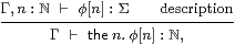
A predicate Γ, n:ℕ⊢φ[n] is called a description
if it is uniquely satisfied, i.e.
| Γ ⊢ (∃ n.φ[n]) ⇔ ⊤ and Γ, n,m:ℕ ⊢ (φ[n]∧φ[m]) ⇔ (φ[n]∧ n=m). |
We shall refer to these two conditions as existence and uniqueness respectively. Using inequality, uniqueness may be expressed as
| Γ ⊢ (∃ m,n.φ[m]∧φ[n]∧ n≠ m) ⇔ ⊥. |
Definition 9.4 Any description entitles us to introduce its numerical witness,
|
the elimination rule being the singleton
| n:ℕ ⊢ |
| ≡ (λ m.m=n) :Σℕ, |
which is easily shown to be a description. Then the β- and η-rules are
| Γ, n:ℕ ⊢ (n=the m.φ[m]) ⇔ φ[n] and n:ℕ ⊢ (the m.m=n) = n. |
The restricted λ-calculus, together with the lattice structure and primitive recursion in Remarks 2.4–2.5 and these rules, is called the description calculus.
Lemma 9.5
Let Γ, n:ℕ ⊢ ψ[n]:Σ be another predicate.
Then, assuming these rules,
Proof By Lemma 9.2, ψ(the n.φ[n]) ⇔ ∃ m.ψ[m]∧(m=the n.φ[n]), which is ∃ m.ψ[m]∧φ[m] by the β-rule for descriptions. ▫
[The statement and proof of the following result were incorrect in the published version of this paper; this version appeared as Lemma E 2.8. It turns recursion at type ℕ into recursion at type Σℕ, as part of the process of bringing descriptions (the m.) to the outside of a term.]
Lemma 9.6 Γ ⊢ r n ≡
rec(n, z, λ n′ u. s(n′,u)) = the m.ρ(n,m) , where
|
Proof The base case (in context Γ) is
|
The induction step, with the hypothesis λ m′.ρ (n, m′) = λ m′.(m=r n′), is
|
So Γ, n:ℕ ⊢ λ m.ρ(n,m) = λ m.(m=r n). ▫
Hence we have the analogue of Proposition 8.10 for descriptions.
Proposition 9.7
Any term Γ⊢ a:X in the description calculus is provably equal
Proof By structural recursion on the term a, in which Lemmas 9.2, 9.5 and 9.6 handle the non-trivial cases. ▫
Remark 9.8 As in Remark 8.3 for focus,
we must be careful about the scope of the description,
— how much of the surrounding expression is taken as the formula ψ?
For F:ΣΣ, does
| F(ψ(the n.φ[n])) reduce to F(∃ n.φ[n]∧ψ[n]) or to ∃ n.φ[n]∧ F(ψ[n]) ? |
Once again, it does not matter, as they are equal, so long as φ is a description. Otherwise, they are different if F(⊥) ⇔ ⊤, for example if F≡λσ.⊤ or (in set theory) F≡¬.
Remark 9.9 The theory of descriptions was considered by Bertrand Russell
[RW13, Introduction, Chapter III(1)]
[vH67, pp 216–223]
[GG00, Section 7.8.4].
The theme of his development is that the n.φ[n] is incomplete:
it acquires a meaning only when embedded in a predicate ψ,
as in Lemma 9.5.
(This came out of his dispute with Hugh McColl and Alexius Meinong
regarding grammatically correct noun-phrases that don’t denote
[GG00, Section 7.3].)
Russell defined
| ψ[the n.φ[n]] as ∃ n. ψ[n]∧φ[n]∧(∀ m.φ[m]⇒ n=m), |
incorporating the condition of unique satisfaction as a conjunct in this predicate. He used an inverted iota for the description operator.
So long as φ is a description, Russell’s definition is equivalent to our β-rule, but ∀ is not a symbol of our calculus — for the reasons that we set out in Section 1.
Gottlob Frege had treated the description operator as an everywhere-defined function-symbol, written \ [Fre93, §11] [GG00, Section 4.5.6]. He therefore had to make a case-distinction, in which \φ returns the member of a singleton class, but the class itself if it is not a singleton. A 1960s logic textbook that I prefer not to advertise assigns [the value] 0 [to any expression] the n.φ[n] whenever φ fails either of the conditions for being a description, with the result that
is true since 0=0 (and this book had two authors).
As we have observed, if we are allowed to write the n.φ[n] without φ satisfying the condition, then all sorts of mathematical transformations that we would normally expect to be able to make become invalid. Frege’s case-distinction is not computable — we have first to determine the cardinality of the class, which may involve answering an arbitrarily difficult mathematical question. It also illustrates the untyped nature of his calculus (which was a part of its downfall): if we introduce a=the x.φ[x], we at least expect φ[a] to be meaningful (though maybe false if φ is unwitnessed), which it is not if a is a set. Even Russell’s good intentions of enforcing the description property are frustrated by his object-language implementation, as it may result in some larger formula becoming true contrary to common sense.
Giuseppe Peano [Pea97] [GG00, Section 5.4.3] had also recognised the incomplete nature of description-phrases in mathematics. On the other hand, he required the predicate to be a description as a premise to the definition of the operator, for which he wrote ι, using ι a for our {a}. So, the condition of unique satisfaction is part of the meaning in a meta-logical way: if the author has written the n.φ[n] anywhere, there is an implicit claim that φ has been proved to be a description, and this fact may be re-used anywhere in the argument. This is the point of view that we have taken: it is a side-condition on the well-formedness of the expression. At the very least, it documents the fact, and to rely on some exceptional behaviour is hacking.
Whilst Russell’s extension of Peano’s iota to non-descriptions is questionable, from our denotational point of view, he did take the technical analysis a step further by considering the scope of the expression, as in Remark 9.8.
[Claus-Peter Wirth felt that I have done a dis-service to Peano here, and drew my attention to [Pea97, §22]. In my own translation of the text and the notation, this reads
..., let α be a class containing a single member, that is:We call this member ια. That is
- there is an α, and
- whenever we take two things x and y from α, these must always be equal.
This definition really gives a meaning to the whole formula x=ια, and not just to the combination ια.
(∃ x.x∈ α), (∀ x y.x, y∈ α⇒ x=y) ⊢ (x=ια) ⇔ (α=
⎧
⎨
⎩x ⎫
⎬
⎭). Any proposition containing ια is reducible to the form ια∈φ, where φ is a class, and hence to α⇒φ, from which the sign ι has disappeared, even though we can’t form an equality whose first member is ια and the second is a group of known symbols [i.e. define ια in terms of known symbols].
This contains at least a hint of Proposition 9.7, long before other people had the syntactic or proof-theoretic tools to prove normalisation theorems.]
The obvious way to find the n.φ[n] is to search for the least n that satisfies φ[n]. In order to be sure that it is the least, we must check ¬φ[m] for each m< n along the way.
Definition 9.10 Γ⊢α:Σ is said to be
complemented or decidable if there is some (unique)
Γ⊢β:Σ such that α∧β⇔⊥ and
α∨β⇔⊤. We write ¬α for β.
| Γ, n:ℕ ⊢ φ[n] ≡ ψ[n]∧∀ m< n.¬ψ[n] |
Remark 9.12
The search operator µ is usually defined without the existence and
decidability conditions (ψ being replaced by a partial function
ψ:ℕ⇀2), and then itself defines a partial function,
i.e. a program that need not terminate.
The universal property of ℕ, as formulated in category theory by Bill Lawvere, is known in logic as primitive recursion. Adding the search operation gives general recursion. This is known to be properly more powerful, as functions can be defined using it that grow much faster than is possible using primitive recursion alone. Since, as we show in the next section, definition by description in ℕ is equivalent to sobriety, the way that we described in Section 1 of defining computational values via observations really does define bigger numbers than we could obtain directly. (At any rate, it defines bigger functions, but since functional notation such as 10n and its generalisations are essential for writing big numbers, it is widely argued that general recursion does indeed define bigger numbers.)
Although general recursive functions are partial, we would prefer to treat them as total functions ℕ→ℕ⊥ into the lift. This object may be seen as a closed subspace of Σℕ, but its construction in abstract Stone duality makes rather serious use of the lattice structure on Σ [D][F].
Remark 9.13
When we add subspaces to our calculus in [B],
we find that a predicate that is a description on the subspace of interest
may no longer satisfy the existence and uniqueness criteria
on the ambient space.
Conversely, any predicate becomes a description when restricted to
the (possibly empty) locally closed subspace
defined by the ⊤ and ⊥ equations in Definition 9.3.
Nevertheless, it turns out that the n.φ[n] may be manipulated
on the subspace by using the β-rule as we have given it,
but on the ambient space,
even though this it is not a well formed expression there.
Although the reduction may result in expressions with different meanings
on the ambient space, they agree as intended on the subspace.
In this section we prove that focus and description are inter-definable, for the natural numbers. In the following notation, we need to show that φ is a description iff P is prime.
Lemma 10.1 This is a retraction,
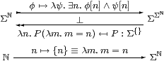
cf. the connection between {} and η in [BW85, Lemma 5.1.3] and Lemma C 6.12. ▫
[In fact there is an adjunction or coclosure as shown, since
|
using the Euclidean principle (Remark 2.4) and the substitution rule for equality.]
First, we characterise the image of Σℕ↣ΣΣℕ.
Lemma 10.2 Γ⊢ P:Σ2ℕ is of the form
λ ψ.∃ n.φ[n] ∧ ψ[n]
for some Γ⊢φ:Σℕ
iff it preserves ∃ℕ.
In this case, φ=λ n.P(λ m.n=m).
Proof Suppose that P preserves ∃. Then
|
by the Euclidean principle (Remark 2.4). The other way is easy. ▫
For the rest of this section, P and φ will be related in this way.
Lemma 10.3 P preserves ⊤ iff φ satisfies the existence condition,
and P preserves ∧ iff φ satisfies the uniqueness condition.
Proof For the first, observe that P⊤ ⇔ ∃ n.φ[n]. For the second, if φ[n1]∧ψ1[n1] and φ[n2]∧ψ2[n2] then n1=n2=n by uniqueness. ▫
Proposition 10.4 If P is prime then φ is a description,
and the n.φ[n] satisfies the rules for focusP
(Definition 8.2).
Proof As P is prime, it preserves ⊤, ∧ and ∃ because its double exponential transpose is a homomorphism, in particular with respect to ⊤, ∧ and ∃, as in Proposition 5.5. Also, P=λψ.∃ n.φ[n]∧ψ[n] by the Lemma, so Pψ⇔ψ[the n.φ[n]], which means that the β-rules agree. For the η-rules,
| φ= |
| ≡(λ m.m=n) iff P=thunkn≡λψ.ψ[n], |
which are respectively a description and prime, and then (the m.φ[m])=(focusP)=n. ▫
Corollary 10.5
Any overt discrete object that admits definition by description is sober.
In particular, all sets and all objects of any topos are sober.
▫
The converse is the case X=ℕ of Theorem 5.7, that if H:Σℕ→ΣU is a frame homomorphism (i.e. it preserves ⊤, ∧ and ∃) then it is an Eilenberg–Moore homomorphism. Of course, we showed that for LKLoc, by re-interpreting results from the literature, not for our abstract calculus. The proof below depends on (primitive) recursion, so only applies to ℕ rather than to discrete overt spaces in general, although when the whole theory is in place the result will hold for them too. [It is easy to show that if φ is a description then P preserves ⊤, ⊥, ∧ and ∨; then it is prime by Theorem G 10.2.]
But before considering ℕ we have to deal with 2≡{0,1}. As we did not ask for this as a base type in Section 2, ψ:Σ2 may be replaced by <ψ0,ψ1>∈Σ×Σ, and similarly for the type of P. (Alternatively, one could formulate a result with ψ:Σℕ to capture the same point.) See Section B 11 for further discussion of disjoint unions in abstract Stone duality.
Proposition 10.6 Let α:Σ be decidable,
with β⇔¬α (Definition 9.11). Then
| P ≡ λψ.(α∧ψ[0])∨(β∧ψ[1]) |
is prime. This justifies definition by cases: (if α then 0 else 1)≡focusP.
Proof Let Pαβ be the obvious generalisation, so
| γ∧ Pαβ = P(γ∧α)(γ∧β) |
by distributivity. The equation that we have to prove for Definition 8.1 may be written
| (α∨β)∧F Pαβ ⇔ (α∧F P⊤⊥) ∨ (β∧F P⊥⊤). |
By the Euclidean principle (Remark 2.4) and the lattice laws, we have
|
Lemma 10.7 For any description φ, we define, by primitive recursion,
| φ≥[0]≡⊤ φ>[n]≡φ≥[n+1]≡φ≥[n]∧¬φ[n] |
| φ<[0]≡⊥ φ≤[n]≡φ<[n+1]≡φ<[n]∨φ[n]. |
Then φ<[n] has the properties of the ordinary arithmetic order, that is, (the m.φ[m])< n, and similarly for the others. ▫
Proposition 10.8 If φ is a description then P is prime,
and focusP satisfies the rules for the n.φ[n].
Proof The idea of the proof is to define a permutation f:ℕ≅ℕ that cycles the witness to 0 and any smaller values up by 1, leaving bigger numbers alone. The function f itself is defined by (cases and) primitive recursion, but it only has an inverse with general recursion. Let
| f(n) ≡ | ⎧ ⎪ ⎨ ⎪ ⎩ |
| δ(n,m) ≡ | ⎧ ⎪ ⎨ ⎪ ⎩ |
|
so δ(n,m) ⇔ f(n)=m. The operations Σf and I, defined by
|
are mutually inverse, because, by expanding disjunctions,
|
Thus Σf is a homomorphism, as is its inverse I by Proposition 3.5. But so too is evaluation at 0, so
| ψ ↦ θ[0] ≡ ∃ n.δ(0,n) ≡ ∃ n.φ[n]∧ψ[n] |
is a homomorphism, and P is prime. The β- and η-rules agree as before. ▫
Remark 10.9
Sobriety says that the functor Σ(−):Cop→A
in Definition 4.1 is full and faithful.
But in this proof we only used the fact that it reflects invertibility,
so it suffices to assume that ℕ is replete.
Then f−1 is the diagonal mediator that is provided by
the orthogonality property
[Hyl91, Tay91].
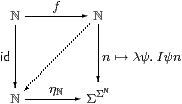
Corollary 10.10 H:Σℕ→ΣU is an Eilenberg–Moore
homomorphism iff it preserves ⊤, ∧ and ∃. ▫
This result can be extended from ℕ to higher types on the assumption of the continuity axiom (Remark 2.6). Hence there is a version of Theorem 5.7 that links the notions of homomorphism and sobriety that we have introduced entirely abstractly using the λ-calculus with those that arise from the ℕ-indexed lattice structure in Remarks 2.4ff. Although the proof would only require one more section, it begins to make serious use of domain-theoretic ideas, and so properly belongs in a discussion of that subject [F][G]. Besides, surprisingly much progress can be made with the development of topology without the extra axiom.
We saw in the previous two sections that the new focus operator is equivalent to definition by description. This is more familiar, both in the sense of tradition, but also in that the requirements on its data are more idiomatic: a predicate with a unique numerical solution, rather than a term of type Σ2 X satisfying a strange equation. Indeed, this calculus seems to be a useful denotational basis for both mathematical and computational investigations: it plays a similar role to that of the class of total recursive functions, whilst being better both as a type theory and for computation.
As it stands, it does not meet the needs of mathematicians, who expect to be able to form subtypes by means of the axiom of comprehension and other constructions such as disjoint sums. Such subtypes, specified by a comprehension-like operation, but equipped with the subspace topology, will be added to the category in [B]. However, this is ignored by computation, i.e. by the reduction rules for the terms.
Topological ideas such as compact Hausdorff spaces are studied in [C][G], and the partial map classifier or lift X⊥ in [D][F].
Remark 11.1 For high-level computation, on the other hand, the calculus is already
a serviceable functional programming language.
It has as
Following Peter Landin [Lan64], it is useful to “sugar” λ-application (λ x.φ)a or plain substitution [a/x]*t, with syntax such as
| let x=a in t or t where x=a. |
The Y-combinator that we derived from the continuity axiom in Remark 2.6 provides recursively defined procedures. So
| letrec φ(x1,⋯,xn)=F in t, |
in which φ may be used in F as well as in t, is encoded as
| let φ = ∃ n. rec (n, ⊥, λ m φ x1⋯ xn. F) in t. |
The body F may contain the “recursive call” φ and its recursive arguments x1,⋯,xn; these are the variables bound by the λ within rec. The numerical variables n and m count the depth of the recursion, but their values are forgotten by ∃ n.
The development of mathematical and topological structures contributes Floyd–Hoare reasoning and special types such as X⊥ to the programming applications. However, by using mathematical intuitions to construct ℝ [I]and other objects, it will also provide methods of programming (i.e. algorithms) for problems where no order of evaluation is naturally apparent.
Remark 11.2 How could we then compile such a program?
As we have understood the calculi in this paper denotationally, let us first clarify what we mean by compilation and execution. In, for example, elementary algebra, we use the rules (such as distributivity) in whatever fashion seems best, to simplify the given complicated expression into a denotationally equivalent one that lies within a subclass of preferred forms. In doing this, we choose some amongst all valid reduction paths.
The objective may be “full” execution, in which we are satisfied with nothing less than an explicit number (assuming that the expression is of type ℕ), and thereby risk non-termination. Alternatively it may be to re-express the program in some simpler language, removing high-level features, but without actually doing the iterations. This translation is called compilation, and is required always to terminate. Sometimes compilation may use η-rules and reverse β-rules that would not be used in an execution strategy.
Remark 11.3 Without loss of generality, the term to be compiled is of type Σ,
since terms of higher type may be applied to free variables,
and a numerical term Γ⊢ t:ℕ
may be handled as Γ,m:ℕ⊢ m=t:Σ.
For example, a numerical function f:ℕ→ℕ
is treated in the form of its graph, n,m:ℕ⊢ m=f(n):Σ.
[Terms of other types are obtained by enclosing logical ones in
the n. or
λ x.]
Lemmas 9.2, 9.5 and 9.6 eliminate embedded descriptions and recursion of numerical type in favour of additional existentially quantified variables, so the numerical sub-terms that remain are ordinary expressions.
Suppose at first that the term doesn’t involve disjunction or recursion: any such sub-term is replaced by a logical variable and will be handled separately.
Since we have a fragment of the simply typed λ-calculus with some constants, the term strongly normalises. This eliminates λ-abstraction and application, which is a desirable property of our compiler, as both Abstract Stone Duality and the Continuation-Passing Style introduce numerous “administrative” λ-expressions of the form λφ.φ[a].
Any existential quantifiers may be moved to the front by renaming the bound variables (this uses the Frobenius law to get past ∧). What remains is either ⊤, ⊥, or a conjunction of sub-terms, each of which is either
The entire term may be existentially quantified over some numerical variables, effectively “hiding” them. This is a pure Prolog clause (apart from the free logical variables).
The numerical equations may be normalised by unification. The occurs check must be made, since logically (∃ n.n=f(n))≡⊥ if f is any non-trivial numerical expression in which the variable n is free. The result of unification serves as a pattern that the free numerical variables must satisfy; the pattern is incorporated into the head of the clause, and many of the hidden variables are eliminated in this process. The body consists of the other logical conjuncts.
We restore disjunction to the language by introducing a Prolog predicate-symbol for each ∨ sub-term, with a clause for each branch. In order to be denotationally equivalent to the original term, these disjuncts must in general be executed in parallel. This is because they may fail either finitely (because of a clash in unification) or infinitely by non-termination, whereas ∨ is meant to be commutative. In practice, the branches are usually guarded by patterns, all but one of which fail straight away.
The term rec(n,Z,λ m u.S) is treated like the disjunction
| (n=0∧ Z)∨(∃ m.n=m+1∧ S(m,u)) |
but with an actual link to rec(m,Z,λ m u.S) in place of u. The circular translation from programming language to our calculus and back therefore simply introduces a hidden variable n that counts the depth of the recursion. (There is a disjunct ⊥ that is redundant.)
For the most part, logical variables in the main program are bound to Prolog procedures, any free ones being (illegally) undefined procedure names. However, recursion at type ΣΣℕ or higher types does involve passing logical arguments to recursive procedures. In simple cases, this may be done by Gödel-numbering them, and in fact it is not difficult to write a self-interpreter for and in pure Prolog.
Remark 11.4
Turning from low- to high-level programming, what can we make
of Thielecke’s force operator? In our treatment, we insisted that
focus be accompanied by its side condition (that it only be applied
to primes), so maybe we are unable to interpret control operators.
But the difference is merely that we have investigated SC,
which includes general recursive function,
and argued that it should be used in place of C,
which only has primitive recursion.
The category HC with control operators is still there,
and HC≅HSC.
Its terms are interpreted contravariantly in C,
by means of a λ-translation which, when written on paper,
may seem complicated [Fis93, Section 4],
but is dissolved away by our λ-normalising compiler.
John Reynolds has given a nice historical survey of mathematical and computational calculi that use continuations [Rey93]; for a formal introduction to control operators, you should see the work cited there. Here, we shall just say something about the consequences of dropping the primality side-condition, by way of an introduction addressed to mathematical readers. Note that the programming language for HC that we’re about to describe is to be translated into the sober calculus, and is not an extension of it.
In return for allowing force to be used without restriction, we have to constrain the reduction rules in general, i.e. to impose an order of evaluation. We choose call by value, in which the argument a is reduced before the β-redex (λ x.φ)a, and unapplied abstractions λ x.φ are not reduced at all.
This means, in particular, that the argument of φ(forceP) gets evaluated before φ, turning the expression into Pφ. However, we must specify how much of the enclosing expression φ is to be consumed by this reduction. We do this by introducing another keyword, label, as a delimiter (it has no computational effect in itself). Since force may occur repeatedly, we must name the label that delimits each force. Assuming that neither F nor φ can be reduced on its own,
| F(labelk φ (forcek P)) reduces to F(Pφ). |
What has happened here, in programming terms? The part of the continuation (φ) that is bracketed by label and force has been given to P as an argument. Because of the call-by-value rules, φ does not get executed until P puts it into an active position in front of an argument. P may also duplicate or lose φ. When it has finished, P does not return in the normal way to its calling context (φ), but to F, i.e. to the position of the matching label. In other words, forcek jumps to labelk. Unless, that is, φ gets executed and itself performs a different jump.
Remark 11.5 Our compiler translated disjunction into alternative
Prolog clauses, which ought in general to be executed in
parallel. If, however, one branch fails finitely, it can
back-track to the point of choice, and proceed with another option.
Continuations provide the natural way in which to do this. Instead of having a single calling context φ to which it always returns normally, a sub-program that has a notion of finite failure can be supplied with two continuations, φ+ and φ−, which it may invoke respectively in the event of success and failure [Hay87, Thi01]. This translation is not the one that we obtain from disjunction (cf. Proposition 10.6), but does fall naturally out of the interpretation of coproducts (disjoint unions) in Section B 11.
Remark 11.6 There are several reasons why pure Prolog should arise as
the intermediate or object language of our compiler,
that is, that we use logic rather than functional programming.
Primarily, it is that we chose ΣX rather than X⊥
our basic type constructor.
Then terms Γ→ΣX are relations,
whereas those Γ→ X⊥ are partial functions.
However, it is a curious feature of Prolog that single clauses are static: the control and data-flow only acquire a direction when the clauses are put together into a whole program. This may perhaps be connected with the fact that it is a natural target of the continuation-passing style, i.e. that we are translating high-level programs that are themselves ambivalent about their direction.
The papers on abstract Stone duality may be obtained from