


Marshall Stone showed us that we should always look for the topology on mathematical objects, and ASD was called after him partly because this is its fundamental message too. However, our discussion of infinitary joins and computable bases in Definitions 1.5 and 3 has shown that this topology may still be the discrete one, i.e. that we need sets after all. Since we have no sets as such, we think of these objects as “discrete” spaces. In ASD we take this particular word to mean that there is an internal notion of equality, but the logical structure that we need to express the join is existential quantification.
Definition 4.1 An object N∈obS is discrete if there is a pullback
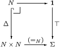
i.e. the diagonal N↪ N× N is open. We may express this symbolically by the rule
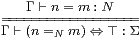
for Γ⊢ n,m:N,
|
The (=) above the line denotes externally provable equality of terms of type N, whilst (=N) below the line is the new internal structure. Categorically, (n,m):Γ→ N× N and !:Γ→1 provide a cone for the pullback iff (n =N m) ⇔ ⊤, and in just this case (n,m) factors through Δ, i.e. n=m as morphisms.
We also write {n}:ΣN for the singleton predicate λ m.(n=N m) but {|n|}:List N for the singleton list.
Beware that this notion of discreteness says that the diagonal and singletons are open, but not necessarily that all subspaces of N are open. For example, the Gödel numbers for non-terminating programs form a closed but not open subspace of ℕ [D, F], because the classically continuous map ℕ→Σ that classifies it is not computable (Definition 1.6).
Definition 4.2
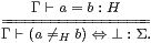
Similarly, an object H is Hausdorff if

is closed, i.e. co-classified by (≠H):H× H→Σ, so
for Γ⊢ a,b:H,
|
Notice that equality of the terms a,b:H corresponds to a sort of doubly negated internal equality, so this definition carries the scent of excluded middle. Like that of a closed subspace, it was chosen on the basis of topological rather than logical intuition. As we saw in Example 2 discrete spaces need not be Hausdorff.
Definition 4.3
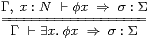
An object N∈obS is overt if Σ!N
(where !N is the unique map N→1)
has a left adjoint, ∃N:ΣN→Σ,
with respect to the intrinsic order (Definition 3.7).
Then
for Γ⊢ σ:Σ, φ:ΣN,
|
where we write ∃ x:N.φ x or just ∃ x.φ x for ∃N(λ x:N.φ x). The Frobenius law,
| σ∧∃ x.φ x ⇔ ∃ x.σ∧φ x |
may be derived from the Phoa principle (Axiom 3.6), and Beck–Chevalley is also automatic (Section C 8). The lattice dual of this definition is the subject of the next section.
Axiom 4.4
S has a natural numbers object ℕ, i.e. an object that
admits primitive recursion at all types, and so is discrete and
Hausdorff. We also require ℕ to be overt.
In order to prove the results that we expect by induction, equational hypotheses must be allowed in the context Γ of each judgement. See [E, §2] for a discussion of this.
Remark 4.5 Since the object N over which the codes
range is discrete, its intrinsic order ≤ is trivial
(Lemma C 6.2). However, the structure (N,0,1,+,⋆) of an abstract basis is,
at least morally, supposed to be
that of a distributive lattice (Remark 1.8).
But this is an “imposed” structure,
i.e. one that is only defined by the explicit specification of
(0,1,+,⋆),
rather than by its relationship to the other objects in the category.
We are completely at liberty to consider functions that preserve,
reverse or disregard the associated imposed order relation ≼
that may be defined from + and ⋆ (Definition 13.10).
Indeed, the need to use conditions that are contravariant with respect to
the natural order was precisely the reason for distinguishing between
N (or |ΣX|) and ΣX in Remark 3.9.
We typically use the letter N for an overt discrete object, as its topological properties are like those of the natural numbers (ℕ), though the foregoing remarks do not give it either arithmetical or recursive structure. So when we write (βn) for the basis of open subspaces, we intend a family, not a sequence. The use of the letter N is merely a convention, like K for compact spaces; the letter I (for indexing set) is often used elsewhere in the situations where we use N below, but it has acquired another conventional use in abstract Stone duality (cf. Lemma 7.4). The notation and narrative may give the impression of countability, but bases in the classical model (Remark 3.1(a)) may be indexed by any set, however large you please. Nevertheless, I make no apology for this impression, as I consider ℵ1 and the like to have no place in topology. I also suspect that occurrences of “sequences” and “countable sense subsets” in the subject betray the influence of objects whose significant property is overtness and not recursion.
Theorem 4.6 The full subcategory of overt discrete spaces is a pretopos,
i.e. we may form products, equalisers and stable disjoint unions of
them, as well as quotients by open equivalence relations
(Section C 11). If the “underlying set” functor in Remark 3.10
exists, as in the classical models LKSp and LKLoc,
then the overt discrete spaces form
an elementary topos [H]. ▫
The combinatorial structures of most importance to us, however, are the following:
Theorem 4.7 Assuming a “linear fixed point” axiom
(that any F:ΣU→ΣV preserves joins of ascending sequences),
every overt discrete object N generates
a free semilattice K N and a free monoid List N in S,
which satisfy primitive recursion and equational induction schemes,
and are again overt discrete objects [E]. ▫
This result is easy to see in the two cases of primary interest, namely the classical and term models (Remark 3.1). In the classical ones (LKSp and LKLoc), overt discrete spaces are just sets with the discrete topology, and form a topos. In this case the general constructions of List (−) and K(−) are well known: K N is often called the finite powerset.
Remark 4.8 In the term model, on the other hand,
we shall find in Section 8 that
ℕ itself is adequate to index the bases of all definable objects.
Moreover, any definable overt discrete space N is in fact the
subquotient of ℕ by a some open partial equivalence relation
(Corollary 9.2).
This both allows us to construct List (N) and K(N),
and also to extend any N-indexed basis to an ℕ-indexed one.
There is, therefore, no loss of generality in taking all bases in this
model to be indexed by ℕ, if only as a method of
“bootstrapping” the theory.
To construct List (ℕ), we could use encodings of pairs, lists and finite sets of numbers as numbers. However, it is much neater to replace ℕ with the set T of binary trees. Like ℕ, T has one constant (0) and one operation, but the latter is binary (pairing) instead of unary (successor), and the primitive recursion scheme is modified accordingly. Hence T≅{0}+T×T≅List (T), whereas ℕ≅{0}+ℕ. The encoding of lists in T has been well known to declarative programmers since Lisp: 0 denotes the empty list, and the “cons” h::t is a pair.
Membership of a list is easily defined by list recursion, as are existential and universal quantification, i.e. finite disjunction and conjunction.
|
Notation 4.9
The notation that we actually use in this paper conceals the
preceding discussion.
The letter N may just stand for T in the term model,
but may denote any overt discrete space.
So, in the classical models, N is a set, or an object of the base topos,
equipped with the discrete topology.
We use Fin(N) to mean K(N) or List (N) ambiguously. Since they are respectively the free monoids on N with and without the commutative and idempotent laws, this is legitimate so long as their interpretation also obeys these laws. But this is easy, as the interpretation is usually in ΣX, with either ∧ or ∨ for the associative operation. In fact, these two interpretations in ΣΣN are jointly faithful [E].
We are now ready to state the central assumption of this paper.
Axiom 4.10 The Scott principle:
for any overt discrete object N,
| Φ:ΣΣN, ξ:ΣN ⊢ Φξ ⇔ ∃ℓ:Fin(N).Φ(λ n.n∈ℓ) ∧ ∀ n∈ℓ. ξ n. |
Notice that the Phoa principle (Axiom 3.6) is the special case with N=1 and so K(N)={0,1}, whilst the “linear fixed point” axiom in Theorem 4.7 can easily be shown to be equivalent to the case N=ℕ. More generally, the significance of this axiom is that it forces every object to have and every map to preserve directed joins (which we have yet to define), and so captures the important properties that are characteristic of topology and domain theory.
Remark 4.11 The lattice ΣX has
intrinsic M-indexed joins, for any overt discrete object M.
These are given by λ x.∃ m:M.φm x,
and are preserved by any Σf
(Corollary C 8.4).
In speaking of such “infinitary” joins in ΣX, we are making no additional assertion about lattice completeness: there are as many joins in each ΣX as there are overt objects, no more, no fewer. In particular, there are not “enough” to justify impredicative definitions such as the interior of a subspace, or Heyting implication (though these can be made in the context of the “underlying set” assumption in Remark 3.10 [H]).
Moreover, we use the symbol ∃ to emphasise that our joins are internal to our category S, whereas those in locale theory (written ⋁) are external to LKLoc, involving the topos (Set) over which it is defined. This distinction will, unfortunately, become a little blurred because of the need to compare the ideas of abstract Stone duality with those of traditional topology and locale theory. This happens in particular in the definition of compactness (Definition 5.2), the way-below relation (Definition 2 and Remark 6.14) and the characterisation of finite spaces (Theorem 9.10)
Remark 4.12 When we use M-indexed joins,
we shall need M to be a dependent type,
given, in traditional comprehension notation
(not that of [B]), by
| M ≡ {n:N ∣ αn} ⊂ N, |
where αn selects the subset of indices n for which φn:ΣX is to contribute to the join. In practice, this subset is always open, so αn:Σ. The sub- and super-script notation here (and in [H]) indicates that φn typically varies covariantly and αn contravariantly with respect to an imposed order on N. Indeed there would be no point in using αn to select which of the φs to include in the join if this had to be an upper subset, as the result would always be the greatest element, whilst it is harmless to close the subset downwards.
This means that, when using the existential quantifier, we can avoid introducing dependent types by defining
| ∃ m:{n:N ∣ αn}.φm as ∃ n:N.αn∧φn. |
In Section 6 we shall refer to terms like αn of type Σ as scalars and those like φn of type ΣX as vectors.
Definition 4.13 A pair of families
| Γ, s:S ⊢ αs:Σ, φs:ΣX |
indexed by an overt discrete object S is called a directed diagram, and the corresponding
| ∃ s.αs∧φs |
is called a directed join (cf. Definition 1), if
In this, αs∧αt means that both φs and φt contribute to the join, so for directedness in the informal sense, we require some φs+t to be above them both (covariance), and also to count towards the join, for which αs+t must be true.
Although the letter S stands for semilattice, in order to allow concatenation of lists to serve for + (and the empty list for 0), we do not require this operation to be commutative or idempotent (or even associative).
Remark 4.14
By the Scott principle, any Γ⊢ F:ΣΣX
preserves directed joins, in the sense that
| F(∃ s.αs∧φs) ⇔ ∃ s.αs∧ Fφs. |
Notice that F is attached to the “vector” φs and not to the scalar αs, since the join being considered is really that over the subset M≡{s ∣ αs}.
This is proved in Theorem 9.6, so it is one of the points on which the logical proofs lag some way behind the topological intuitions. Of course, this result could have been used in place of Axiom 4.10, but I feel that I made an important point in [Tay91] by showing how sobriety (actually the slightly weaker notion of repleteness) transmits Scott continuity from the single object ΣN to the whole category.
Remark 4.15 After the separation of directed joins from
finite ones (⊥, ∨),
the behaviour of the latter corresponds much more closely to that
of meets (⊤, ∧).
So, although Scott continuity, strictly speaking, breaks the
lattice duality that we enjoyed in [C, D],
we shall still often be able to treat meets and joins at the same time.
We sometimes use the symbol ⊙ for either of them,
for example in Lemma 16.11.
This means that we can try to transform arguments about open,
discrete, overt, existential, ... things into their lattice duals
about closed, Hausdorff, compact, universal, ... things.
Such lattice dual results seem to be far more common that anyone brought
up with intuitionistic logic or locale theory might expect.
For example, there is a dual basis expansion,
in which ∃∧ are replaced by ∀∨,
but we must leave that to later work.
Lemma 4.16
For Scott continuity, it suffices that the family be inhabited,
in the sense that ∃ s:S.αs⇔⊤,
and have a binary operation + with the properties stated.
In this paper, 0 will typically be the empty list, but in [I, J] we shall use ℚ with max or min, which have no semilattice unit.
Proof Define S′≡ S+{0}, α0≡⊤ and φ0≡⊥. Then
| ∃ s:S′.αs∧φs ⇔ α0∧φ0 ∨ ∃ s:S.αs∧φs ⇔ ∃ s:S.αs∧φs, |
but we need ∃ s:S.αs⇔⊤ for
| F⊥ ⇔ F⊥∧ ∃ s:S.αs ⇔ ∃ s:S.αs∧ F⊥ ⇒ ∃ s:S.αs∧ Fφs. |
Then
|
Inhabitedness is all that we require of a join for it to satisfy the dual distributive or Frobenius law, cf. Lemma 2.7.
Lemma 4.17
If ∃ n.αn⇔⊤ then
φ∨(∃ n.αn∧ψn) =
∃ n.αn∧(φ∨ψn). ▫
The most dramatic effect that Scott continuity has on the presentation of general topology is the way in which it simplifies the notion of compactness, to which we now turn.