


Now we are ready to give a formal introduction to overtness, of which we saw an example in Section 2. This very novel concept is invisible in (even intuitionistic) point–set topology, for a reason that we shall see at the end of this section, so we have to rely entirely on our new calculus.
As our guide, we exploit the lattice duality with the notion of compactness and follow the plan of Sections 8 and 9 as closely as possible. Before going on, you should therefore be sure that you thoroughly understand how the formalism there relates to your own knowledge of compact subspaces, and then refer back to those sections while you read this one.
Under the lattice duality, the theory of open or overt subspaces of (overt) discrete spaces corresponds to that of closed or compact subspaces of (compact) Hausdorff spaces (Theorem 11.20). However, the ambient space that primarily interests us in this paper is Hausdorff, not discrete. More fundamentally, we know that the open and closed phenomena in general topology do not quite match, for example ℕ is overt but not compact, whilst Scott continuity (Axiom 9.1) is about directed joins and not meets.
Since things are not exactly dual we must start from a different place. Motivated by our interest in stable zeroes (Proposition 2.12), we choose the dual of Definition 8.19 for a compact open subspace.
Definition 11.1
A closed overt subspace of a space X
is defined by a pair of terms (◊,ω),
in which ω:ΣX is its co-classifier qua closed subspace
and ◊:ΣΣX is its possibility modal operator
qua overt one.
For ◊ to have this type means that ◊φ is a proposition
(a term of type Σ).
The terms ◊ and ω must be related by the rule that,
for any expression φ:ΣX,
| ◊φ ⇔ ⊥ ⊣⊢ φ ⊑ ω, |
cf. Proposition 2.15. Equivalently (by Axiom 5.6),
| φ x=⇒ω x∨◊φ and ◊ω⇔⊥, |
the first part of which we call relative instantiation, cf. Axiom 5.10. If we want to name the subspace, we write <S> for ◊. The intended meaning of ◊φ is that φ touches the subspace represented by ◊, cf. Proposition 2.2, whereas in Section 8, φ covered ▫.
Proposition 11.2 For a:H, σ:Σ, φ,ψ:ΣH and
θ:ΣH1× H2, ◊ operators obey
Proof It would be a valuable exercise to transcribe the proof of Proposition 8.2 and Exercise 8.20, replacing each symbol with its lattice dual. Uniqueness comes from φ⊑ω′ ⊣⊢◊φ⇔⊥ ⊣⊢φ⊑ω ⊣⊢◊′φ⇔⊥ and Axiom 5.6. The Frobenius law follows from Proposition 5.8 and the substitution property is that for λ-application (Axiom 7.7). Finally, either side of the commutative law is ⊥ iff
| x,y:H, ω1 x⇔ ω2 y ⇔ ⊥ ⊢ φ x y ⇔ ⊥. ▫ |
Remark 11.3
Since ◊ automatically preserves directed joins
(it is Scott-continuous, Axiom 9.1),
it actually preserves all joins,
as in Theorem 2.5.
That’s not quite right:
it preserves joins indexed by other overt objects,
and the same is true of inverse image maps
(f−1, Definition 7.19).
Another way of putting this is that possibility operators commute,
which is what we have just said.
Unlike in the lattice-theoretic or localic language,
we are able to make identical statements about meets and joins.
We resist the temptation to define ◊ simply as an operator that preserves joins because it is not yet clear whether this will still be appropriate in the generalisation envisaged in Remark 7.13.
Example 11.4
As in Proposition 2.15(d) and Example 8.5,
any point defines an overt subspace {a},
with ◊φ≡φ a
and (in a Hausdorff space) ω x≡(x≠ a).
Relative instantiation for this is Lemma 5.9.
Conversely, any term P:ΣΣH that obeys the rules for both modal operators (it is enough that it preserve ⊤, ⊥, ∧ and ∨) is called prime, and arises as P≡λφ.φ a from a unique point a (Section G 10). ▫
Definition 11.5 We say that a:X is a member of the overt subspace, a∈◊,
if, for any φ:ΣX,
| φ a =⇒ ◊φ, or λφ.φ a ⊑ ◊:ΣΣX. |
An overt subspace is said to be inhabited if ◊⊤⇔⊤ (cf. Proposition 3). The existence property (Remark 6.6) provides an actual member of any inhabited overt subspace of ℕ or ℚ (without parameters) and future work will show the same for ℝ.
This notion of membership is another example to which we may apply Notation 7.15 to define a subspace, S≡{x:X ∣ λφ.φ x⊑◊}, cf. Proposition 2.12. Although we have not given any condition on ◊ alone that says when it defines an overt subspace, the two directions of Definition 11.1 now state the containments S⊃ Z and S⊂ Z respectively, in the sense of Definition 7.17.
We sometimes refer to the two-way relationship as the non-singular case. In Section 2 we saw that the singular case arises, for example, from double zeroes of polynomials, where relative instantiation fails but we still have ◊ω⇔⊥.
Proposition 11.6
In the non-singular case,
the two notions of membership for a closed overt subspace agree.
In the singular case,
the overt subspace lies inside the closed one.
Proof S⊂ Z comes from ◊ω⇔⊥ because, if x∈◊ then (putting φ≡ω in the definition) ω x⇒◊ω⇔⊥, so ω x⇔⊥. Conversely, Z⊂ S is relative instantiation, φ x⇒ω x∨◊φ, when ω x⇔⊥. ▫
Proposition 11.7
If d≤ u:ℝ then the interval [d,u]⊂ℝ
is closed overt, with
| ω x ≡ (x< d)∨(u< x) and ◊φ ≡ φ d∨(∃ x:ℝ.d< x< u∧φ x)∨φ u. |
If d< u then ◊φ is just ∃ x:ℝ.d< x< u∧φ x.
The interval [d,+∞) is also closed overt, with
| ω x ≡ (x< d) and ◊φ ≡ ∃ x:ℝ.(d< x)∧φ x, |
and we may define (−∞,u] in a similar way.
Proof By Proposition 9.6, ω co-classifies the closed interval and then ◊ω expands to (u< d)⇔⊥. By Lemma 5.9,
| φ x =⇒ (x< d) ∨ φ d ∨ (d< x). |
The conjunction of this with the similar formula with u gives relative instantiation,
| φ x =⇒ (x< d∨ u< x) ∨ (φ d∨(∃ y.d< y< u∧φ y)∨φ u) ≡ ω x∨◊φ. ▫ |
Examples 11.8 The empty subspace is overt, as is the union of any two
closed overt subspaces, but the intersection may fail to be overt,
even in the simplest cases, {a}∩{b} and [d,u]∩[e,t].
| ▫ |
We shall come back to subspaces shortly, but first let’s look at overt spaces.
Definition 11.9 A space S is overt if it has
an existential quantifier, ∃S,
such that, for x:S and φ:ΣS,
| ∃S⊥⇔⊥ and φ x =⇒ ∃Sφ, |
the latter being called the absolute instantiation rule. In other words, S is a closed overt subspace of itself with ω≡⊥, and any expression of type S is a member of ◊ in the sense of Definition 11.5.
Examples 11.10 The spaces ℕ, ℚ and ℝ are overt
(Remark 5.11).
We write ∃ x:S.φ x for ∃Sφ when S is an overt space, so ∃ x:S.φ x means <S>(λ x.φ x). We sometimes also use ∃ for overt subspaces, i.e. for <S>φ.
Proposition 11.11
Any closed overt subspace is an overt space.
Proof As in Theorem 8.16, given (◊,ω), let C≡{x:X ∣ ω x⇔⊥} with Σ-splitting I:ΣC↣ΣX (Axiom 7.10) and ∃Cψ≡◊(Iψ), so ∃C⊥C≡◊(I⊥C)⇔◊ω⇔⊥. Then, since ω⊑ψ=Iψ, we have, for x:C and ψ:ΣC,
| ψ x=⇒ω x∨◊ψ ⇔ ∃Cψ. ▫ |
The quantifier is justified by Proposition 11.2 and the following rules of inference.
Theorem 11.12 In an overt space, ∃S satisfies the two-way rule on the left,
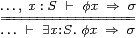
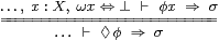
|
where σ:Σ must not involve the variable x. Similarly, ◊ and ω for a closed overt subspace of X satisfy the rule on the right.
As in Remark 8.17, ◊ is a bounded existential quantifier, with which we can reason about members of the subspace as if this were itself a space, cf. Exercise 2.10.
Proof By Axiom 5.6, the rule on the right is
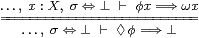 or
or
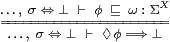
|
which is Definition 11.1. The rule on the left is the special case where ω x ≡ ⊥. ▫
The exact analogue of Theorem 8.9 for the direct image of f:X→ Y when X is overt would require Y to be discrete, whereas we are interested in Hausdorff spaces. Nevertheless, the situation has an extremely important example that explains why Proposition 2.12 gave the closure of the overt subspace ◊.
Notation 11.13 Let <S> be an overt subspace of X, and f:X→ Y. Then
| <f S>ψ ≡ <S>(f*ψ) ≡ <S>(λ x.ψ(f x)) |
is called the direct image of <S>. If a:X is a member of <S> then f a:Y is a member of <f S>, whilst <f S> preserves joins. If S is inhabited then so too is f S because
| <f S>⊤ ⇔ <S>(⊤· f) ⇔ <S>⊤ ⇔ ⊤. |
This doesn’t satisfy the whole of Definition 11.1, because we haven’t defined ω for f S, but this deficit will be rectified in Proposition 12.12 when we have compactness too. In a sense, <f S> is the closure of the image, because it is contained in any closed subspace whose inverse image contains <S>, since <f S>ω⇔⊥ iff <S>(f*ω)⇔⊥.
Example 11.14
The modal operator for the direct image of any map f:ℕ→ X is
| ◊φ ≡ ∃ n:ℕ.φ(f n). |
Let a:X be a member of ◊ (Definition 11.5). For any neighbourhood φ:ΣX of a,
| φ a=⇒◊φ ≡ ∃ n.φ(f n), |
so, since φ was arbitrary, a is an accumulation point of the sequence in the traditional sense, cf. Example 2. Maybe we should have used this name instead of “member” in Definition 11.5. This phenomenon is the dual of Warning 8.4.
Note that, in our usage, the members of a sequence (as well as its limit, if any) are accumulation points of it. However, we are not saying that the sequence has a limit.
Notice that we have only used the topological properties of ℕ, not its arithmetic, recursion or cardinality. Hence the idea generalises to accumulation points of nets of whatever size and shape, so long as they are definable in the underlying calculus.
Remark 11.15
Conversely, every operator ⊢◊:ΣΣℝ
that is definable in the ASD calculus and preserves joins
(◊⊥⇔⊥ and ◊(φ∨ψ)⇔◊φ∨◊ψ)
is of the form ◊φ⇔∃ n:U.φ(f n) for some function
f:U→ℝ with U⊂ℕ open (recursively enumerable).
This will be proved in future work, essentially by applying dependent
choice to Remark 6.11.
Overtness therefore links computability with the Bolzano–Weierstrass theorem
about accumulation points of infinite sets of points.
Returning to subspaces, there are, of course, good reasons why we only find closed compact subspaces of ℝ and not open ones. Despite this and the observation about accumulation points, there are also lots of open overt subspaces, because we have the dual of Proposition 8.7 that any closed subspace of a compact space is compact:
Proposition 11.16
Any open subspace of an overt space is overt.
Proof Let α:ΣX, where X has ∃X. Then
| ◊φ ≡ ∃ x:X.φ x∧α x satisfies ◊φ ⇔ ⊥ ⊣⊢ φ∧α = ⊥ |
and Proposition 11.2, defining an open overt subspace. If a∈α (α a⇔⊤) then a∈◊ (λφ.φ a⊑◊), but in view of the observation about accumulation points, the converse need not hold. Once again, we leave it as an exercise to adapt Propositions 11.2 and 11.11 to open overt subspaces . ▫
Example 11.17 For any d,u:ℝ, the
open interval (d,u)⊂ℝ
is classified by λ x.d< x< u.
More generally, for any ascending real δ and
descending one υ,
the interval (υ,δ)⊂ℝ
is classified by δ∧υ.
These are both overt, where ◊φ is
| <d,u>φ ≡ ∃ x.(d< x< u)∧φ x or <υ,δ>φ ≡ ∃ x.δ x∧φ x∧υ x, |
and are inhabited iff d< u or ∃ x.δ x∧υ x.
Notice that, if d< u, the formula for ◊ is the same as that for the closed interval [d,u] in Proposition 11.7; this is due to the results above concerning accumulation points. ▫
This is the setting for the dual of Proposition 9.13. The ascending real δ is the union of the families of lower bounds of the elements of K. We may form this union because it is indexed by an overt set. Since, for ascending reals, the intrinsic and arithmetical orders agree (Remark 3.10), we have the supremum of K as an ascending real, cf. Remark 2.
Proposition 11.18 For any overt subspace ◊ of ℝ,
| δ d ≡ ◊(λ x.d< x) and υ u ≡ ◊(λ x.x< u) |
provide the supremum δ as an ascending real and the infimum υ a descending one. Since
| ∃ d.δ d ⇔ ∃ u.υ u ⇔ ◊⊤, |
δ and υ are bounded iff ◊ is inhabited. If ◊ is open, classified by α, then α⊑δ∧υ.
Proof By transitivity of < and the Frobenius law for ◊, δ is lower, whilst it is rounded by interpolation and Frobenius, or by Theorem 10.2. Then
| ∃ u.υ u ≡ ∃ u.◊(λ x.x< u) ⇔ ◊(λ x.∃ u.x< u) ⇔ ◊⊤ |
by commutation of ∃ and ◊ (Proposition 11.2(f)) and extrapolation of < (Lemma 5.13). If ◊ is defined from α then α⊑δ∧υ because, by Theorem 10.2,
| α y =⇒ ∃ x z.α x∧(x< y< z)∧ α z =⇒ δ y∧υ y. ▫ |
Exercise 11.19 Develop the notion of overt locally closed subspace
(Axiom 7.10), using
| ◊φ⇔⊥ ⊣⊢ φ∧α⊑ω. |
Show that the half-open, half-closed intervals [e,t), (e,t], [e,δ) and (υ,t] are overt, where
| <[e,δ)>φ ≡ ∃ x.(e< x)∧φ x∧δ x ≡ <e,δ>φ. ▫ |
We have given an account of overt (sub)spaces in the Hausdorff setting because of our focus on real analysis, but this is a seriously one-sided view, because overt discrete spaces play the important role of sets. Since developing this in detail would double the length of this paper, we just mention a couple of points of a topological nature.
Relying, as always, on the duality, we know that the familiar correspondence between closed and compact subspaces takes its strongest form in a compact Hausdorff space (Theorem 8.15). Similarly, we have
Theorem 11.20
The open and overt spaces of an overt discrete space X are in
bijection, by
| α x ≡ ◊(λ y.x=y) and ◊φ ≡ ∃X(φ∧α) ≡ ∃ x:X.φ x∧α x. ▫ |
Corollary 11.21 The following formulations of recursively enumerable
subsets of ℕ agree:
Remark 11.22 This also explains why overtness is invisible in
topology based on points. If a space X has a “set” |X| of points
then |X|↠ X is a surjective continuous function from an overt
discrete space, so X itself is overt by Notation 11.13.