


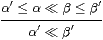
We now introduce the last (g) of our abstract characterisations of local compactness in the Introduction. Recall from Section 2 that any continuous distributive lattice carries a binary relation (written ≪ and called “way-below”) such that
⊥≪γ


|
|
Notation 11.1
We define a new relation n≺≺ m as Anβm.
This is an open binary relation (term of type Σ with two free variables) on the overt discrete object N of indices of a basis, not on the lattice ΣX. It is an “imposed” structure on N in the sense of Remark 4.5.
For most of the results of this section, we shall require (βn,An) to be an ∨-basis for X.
Examples 11.2 (Not all of these are ∨-bases.)
| L≺≺ R ≡ AL BR ⇔ R⊂♯L ≡ ∀ℓ∈ L.∃ℓ′∈ R.(ℓ′⊂ℓ), |
| (ℓ≺≺Σ2 Xℓ′) ⇔ (ℓ≺≺X♯ℓ′). |
Our first result just restates the assumption of an ∨-basis, cf. Lemmas 1.9 and 2.6:
Lemma 11.3 0≺≺ p, whilst
n+m≺≺ p iff both n≺≺ p and m≺≺ p.
Proof A0βp⇔⊤ and An+mβp⇔ Anβp∧ Amβp. ▫
In a continuous lattice, α≪β implies α≤β, but we have no similar property relating ≺≺ to ≼. We shall see the reasons for this in Section 13. But we do have two properties that carry most of the force of α≪β⇒α≤β. We call them roundedness. The second also incorporates many of the uses of directed joins and Scott continuity into a notation that will become increasingly more like discrete mathematics than it resembles the technology of traditional topology.
Lemma 11.4 βn=∃ m.(m≺≺ n)∧βm and
Am=∃ n.An∧(m≺≺ n).
Proof The first is simply the basis expansion of βn. For the second, we apply Am to the basis expansion of φ, so
| Amφ ⇔ ∃ n.Anφ∧ Amβn ⇔ (∃ n.An∧ Amβn)φ, |
since An preserves directed joins (Theorem 9.6). ▫
Corollary 11.5
If m≺≺ n then βm≤βn and Am≥ An. ▫
Corollary 11.6
If m≺≺ n, Am′≥ Am and βn≤βn′,
then m′≺≺ n′.
Proof (m≺≺ n)≡ Amβn⇒ Am′βn′≡(m′≺≺ n′). ▫
Corollary 11.7 The relation ≺≺ satisfies
transitivity and the interpolation lemma:
| (m≺≺ n) ⇔ (∃ k. m≺≺ k≺≺ n). |
Proof Amβn ⇔ (∃ k.Ak∧ m≺≺ k)βn ⇔ ∃ k.Akβn∧ m≺≺ k. ▫
Now we consider the interaction between ≺≺ and the lattice structures (⊤,⊥,∧,∨) and (1,0,+,⋆). Of course, for this we need a lattice basis.
| φ∧ψ = ∃ p q.βp⋆ q∧ Apφ∧ Aqψ and φ∨ψ = ∃ p q.βp+q∧ Apφ∧ Aqψ. |
Proof The first is the Frobenius law, since βp⋆ q=βp∧βq.
The second uses Lemma 4.17: we obtain the expression
| φ∨ψ = ∃ p.Apφ∧(βp∨ψ) |
from the basis expansion φ=∃ p.Apφ∧βp by adding ψ to the 0th term (since A0φ⇔⊤ and β0=⊥) and, harmlessly, Apφ∧ψ to the other terms. Similarly,
| βp∨ψ = ∃ q.Aqψ∧(βp∨βq) = ∃ q.Aqψ∧βp+q. |
The joins are directed because because A0φ∧ A0ψ⇔⊤ and
| (Ap1φ ∧ Aq1ψ) ∧ (Ap2φ∧ Aq2ψ) ⇔ (Ap1+p2φ∧ Aq1+q2ψ). ▫ |
Lemma 11.9 For a lattice basis,
An⊤⇔(n≺≺1), An⊥⇔(n≺≺0) and
|
Proof The first two are Anβ1 and Anβ0. The other two are ∃ p q.An(βp⋆ q)∧ Apφ∧ Aqψ and ∃ p q.An(βp+q)∧ Apφ∧ Aqψ, which are An applied to the directed joins in Lemma 11.8. ▫
Proposition 11.10
The lattice basis (βn,An) is a filter basis iff 1≺≺1 and
|
Proof (n≺≺1)⇔ Anβ1⇔ An⊤, but recall that n≺≺1 for all n iff 1≺≺1.
The displayed rule is Amβp∧ Amβq ⇔ Amβp⋆ q ≡ Am(βp∧βq). Given this, by the Frobenius law and Lemma 11.9,
|
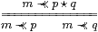
If we don’t have a filter basis, we have to let n “slip” by n≺≺ m, cf. Lemma 2.8:
Lemma 11.11 For any lattice basis,
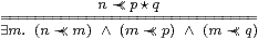
|
Proof Downwards, interpolate n≺≺ m≺≺ p⋆ q≼ p,q, then m≺≺ p,q by monotonicity. Conversely, using Corollary 11.5, if Anβm⇔⊤ and βm≤βp⋆ q then Anβp⋆ q⇔⊤. ▫
The corresponding result for ∨ is our version of the Wilker property, cf. Proposition 1.10 and Lemma 2.7.
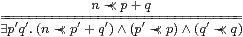
|
Proof Lemma 11.9 with φ≡βp and ψ≡βq. ▫
We shall summarise these rules in Definition 14.1.
There are special results that we have in the cases of overt and compact objects. We already know that 1≺≺ 1 iff the object is compact (cf. Lemma 6.5), but the lattice dual characterisation of overtness cannot be 0≺≺ 0, as that always happens.
Lemma 11.13 If X is overt then
| (n≺≺ m) ⇒ (n≺≺ 0) ∨ (∃ y.βm y) but (n≺≺ 0)∧(∃ x.βn x)⇔⊥. |
Proof φ x⇒ ∃ y.φ y so, using the Phoa principle (Axiom 3.6),
| Anφ ⇒ An(λ x.∃ y.φ y) ⇔ An⊥∨∃ y.φ y∧ An⊤ ⇒ (n≺≺ 0) ∨ ∃ y.φ y. |
Putting φ≡βm,
| (n≺≺ m) ≡ Anβm ⇒ (n≺≺ 0)∨ ∃ y.βm y, |
whilst (n≺≺ 0) ∧ ∃ x.βn x ⇔ ∃ x.Anβ0∧βn x ⇒ ∃ x.∃ n.An⊥∧βn x ⇔ ∃ x.⊥ x ⇔ ⊥. ▫
By a similar argument, we have Johnstone’s “Townsend–Thoresen Lemma” [Joh84],
| (n≺≺ p+q) ⇒ (n≺≺ p) ∨ (∃ y.βq y). |
Corollary 11.14 Given a compact overt object, it’s
decidable whether it’s empty or inhabited, cf. Corollary 5.8.
Proof As (1≺≺1)⇔⊤, the Lemma makes (1≺≺0) and ∃ x.β1 x≡∃ x.⊤ complementary. ▫
Compact overt subobjects are, in fact, particularly well behaved in discrete [E] and Hausdorff [J] objects.
Sections 13–16 are devoted to proving that the rules above for ≺≺ are complete, in the sense that from any abstract basis (N,0,1,+,⋆,≺≺) satisfying them we may recover an object of the category. This proof is very technical, so in the next section we consider a special case, in which the lattice structure plays a much lighter role.