


A subset X⊂ Y of a topological space is said to carry the subspace topology if its open subsets U⊂ X are exactly those of the form U=X∩ V for some open subset V⊂ Y. Since open subsets U⊂ X correspond bijectively to continuous maps φ:X→Σ, there is a more categorical way of saying this:
Remark 2.1 The Sierpiński space Σ
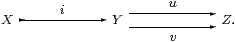
is injective with respect to the inclusion i:
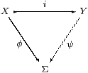
for any continuous map φ:X→Σ, there is some continuous map ψ:Y→Σ such that φ(x) ⇔ ψ(i x).
In the traditional axiomatisation of general topology, the collections of open subsets of X and Y admit arbitrary unions, and i*≡(−)∩ X preserves them. This means that there is a greatest open V≡ i*U⊂ Y such that U=V∩ X, where i*⊣ i*. In particular, if X⊂ Y is the closed subspace complementary to open W⊂ Y, we have V=U∪ W.
As this argument manipulates open subsets and not points, it can be expressed in locale theory. We say that the locale (represented by the frame) A is a sublocale of B if there are monotone functions i*⊣ i* such that i* is a frame homomorphism and2 i*;i*=idA. These can be recovered from the endomorphism j≡ i*;i* on B, which satisfies idB≤ j=j2 and j(b1∧ b2)=j b1∧ j b2. Such a j is called a nucleus. In particular, the nuclei corresponding to the open subspace W⊂ Y and its closed complement are W⇒(−) and W∪(−) respectively.
The lattice of open subsets of a space Y is the exponential ΣY in the category of locally compact spaces and continuous functions, when we equip Y with the Scott topology. In this setting, the inverse image map i* is Σi. However, the monotone functions i* and j need not be morphisms between the objects ΣX and ΣY in this category, as, in terms of the lattices, they need not be Scott continuous.
Many of the features of general topology can be expressed in terms of the λ-calculus that arises from the exponential Σ(−), together with finitary lattice operations and laws [A][C]. Apart from Theorem 3.11 and some Examples, whose purpose is to motivate the ideas, the whole theory will be formulated in these abstract terms: S denotes a category with an internal distributive lattice Σ, of which all powers ΣX exist in S. In fact, even the lattice structure is not used in the main development of the present paper.
Returning to the idea of injectivity, in practice we need to state it with parameters.
Lemma 2.2 The following are equivalent for i:X→ Y:
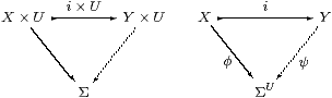
Proof Parts (a) and (b) are exponential transposes of each other, and (c) is the special case of (b) with U≡ΣX and φ≡ηX. Using (b), we obtain I≡ηΣX;Σψ:ΣX→ΣY, as
| I;Σi = ηΣX;Σψ;Σi = ηΣX;ΣηX = id. |
Conversely, ψ≡ηY;ΣI;ΣΣφ;ΣηU satisfies
| i;ψ = i;ηY;ΣI;ΣΣφ;ΣηU = ηX;ΣΣi;ΣI;ΣΣφ;ΣηU = ηX;ΣΣφ;ΣηU = φ;ηΣU;ΣηU = φ. ▫ |
[It follows from this that Σ cannot be injective in the sense of Remark 2.1 in any cartesian closed supercategory of Sob. Any Σ-split subspace of a locally compact spaces is again locally compact (Corollary G 7.6). The object ℕ⊥ℕ is locally compact, being a closed subspace of Σℕ×ℕ, but ℕℕ is not, so the inclusion ℕℕ↣ ℕ⊥ℕ is not Σ-split.
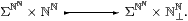
Hence Σ is not injective with respect to the inclusion shown.]
We therefore have a situation in which i:X↣ Y is a subspace (and Σ is injective with respect to it) in a very explicit sense, namely that the way in which open subsets U⊂ X are expanded to V⊂ Y is dictated by a morphism I.
Definition 2.3
i:X→ Y is a Σ-split (mono or) subspace
if there is some morphism I:ΣX→ΣY
such that I;Σi=idΣX.
We shall mark Σ-split monos with a hook like this.
Remark 2.4 The idempotent E≡Σi;I on ΣY
plays a role in our λ-calculus
similar to that of the nucleus j in locale theory,
except that j is uniquely determined by i, whereas E is not.
(So in Section 4
we shall appropriate the name “nucleus” for E.)
Beware, however, that it is not enough for E to be idempotent,
as its epi part Σi must be a (frame) homomorphism.
For locales, this happens iff
| E(φ∧ψ) = E(Eφ∧ Eψ) and E(φ∨ψ) = E(Eφ∨ Eψ), |
though we shall characterise E by a different (λ-)equation in our abstract setting. [In the context of the lattice structure on Σ and Scott continuity, these equations do in fact characterise nuclei in the sense of ASD (Theorem G 10.10).]
ΣY is a continuous lattice, whilst E is Scott-continuous, so its splitting ΣX is also a continuous lattice, and the space X is therefore also locally compact.
Examples 2.5
If a localic nucleus j is Scott-continuous, then it can serve as E.
Otherwise, E may still exist, no longer providing the largest V,
and the map I may extend open subsets from X to Y
in very complicated ways.
Some sublocales need not, however, be represented at all in our formulation.
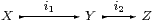
are successively Σ-split subspaces, with
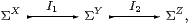
then the composite i1;i2:X↣ Z is Σ-split, with I1;I2:ΣX↣ΣZ.
Compact and overt subspaces are considered in [G][J].
Example 2.6
In set theory, subspaces and open subspaces are the same thing,
but we can still distinguish two roles in the preceding discussion.
Consider a predicate φ∈ΩX,
which classifies the “open” subset U≡{x:X ∣ φ[x]}⊂ X.
This may be expanded from the “subspace” X to Y
using either of the quantifiers:
As for open and closed subspaces, ∃i and ∀i are the left and right adjoints respectively to the inverse image map i*. This analogy between open subspaces and the existential quantifier, and between closed subspaces and the universal quantifier, is explored in [C].
The (Scott) topology on an object Y of Dcpo is determined by its order, and is also the exponential ΣY in that category. However, for a subset X⊂ Y that is closed under directed joins, the Scott topology on X derived from the restricted order need not be the subspace topology.
Example 2.7 (Moggi)
Let Y be the domain of lazy natural numbers,
and X⊂ Y the subset of maximal points ∘ in it,
i.e. the numerals sn0 together with the “top” point ∞,
omitting the points • of the form sn⊥.
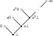
X is the equaliser of the (continuous, recursive) functions f,g:Y⇉ Y for which f(sn 0)≡ g(sn 0)≡ sn+10 but f(sn⊥)≡ sn+1⊥ and g(sn⊥)≡ sn⊥.
The order on X is discrete, as therefore is its Scott topology.
However, its subspace topology is that of the one-point compactification of ℕ: any open subset U⊂ X with ∞∈ U is of the form
| U=({sm0 ∣ m≥ n}⋃ |
| )⋃ F with F⊂{sm0 ∣ m< n} |
for some n. Then V≡{y∈ Y ∣ y≥ sn⊥}∪ F is open in Y with U=X∩ V. Choosing the least such n, the assignment I:U↦ V is monotone, so it is Scott-continuous as there are no non-trivial directed joins to be considered. Hence X⊂ Y is Σ-split, classically. For intuitionistic locale theory, recursion theory and our λ-calculus, the subspace is still an equaliser but the map I is not well defined. ▫
Remark 2.8
The notion of Σ-split subspace has a direct impact on computation
in the λ-calculus associated to the exponential ΣX.
In any category where it is meaningful,
evaluation ev:ΣX× X→Σ is always dinatural in X
with respect to any map i:X→ Y [Mac71, Section IX 4],
i.e. the square from ΣY× X to Σ commutes:
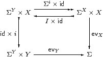
Combining the splitting I with this property, evX is equal to the composite around the other three sides, or, in symbols,
| φ:ΣX, x:X ⊢ φ x ⇔ (Iφ)(i x). (η) |
This equation will later feature as an η-rule of a new λ-calculus for subspaces, based on the axiom of comprehension in set theory. The associated introduction and elimination rules are provided by Σi and I, whilst the β-rule expresses the composite Σi;I ⇔ E:
| ψ:ΣY ⊢ I(λ x.ψ(i x)) = Eψ. (β) |
The importance of the η-rule is that it enables us to evaluate a function φ on a value x in the subspace X by regarding them both as belonging to the ambient space Y instead. Therefore we may reason mathematically in a rich category of subspaces, but execute the computation using the types of the restricted λ-calculus, simply ignoring the new connectives of the comprehension calculus (Section 10).
Remark 2.9 The equation I;Σi=id
says what we require of the open subsets of X and Y,
but does not in fact even force i to be mono on points.
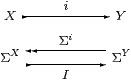
We would actually like it to be regular mono,
i.e. for there to be an equaliser
The corresponding effect on the topologies is
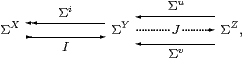
where the fifth map J will be explained in the next section.
Any Σ-split subspace may be expressed in this form, with
| Z≡ΣΣY≡Σ2 Y u≡ηY v≡ηY;ΣI;ΣΣi J≡ηΣY. |
Here the natural transformation ηY is given by the λ-expression y↦λψ.ψ y and is the unit of the adjunction Σ(−)⊣Σ(−). Iteration of the functor Σ(−) obliges us to use the shorthand Σ2 Y.
We have, however, been making an assumption about the category.
Definition 2.10
The maps i ≡ ηX:X→ Y ≡ ΣΣX and I ≡ ηΣX
always satisfy I;Σi=id
(we call the equation ηΣX;ΣηX=id
the unit law),
so X ought to be a subspace of Σ2 X.
The diagram above becomes

with J ≡ ηΣ3 X. Recall from Section A 4 that an object X for which this is an equaliser is called sober. Definition 2.3 and the ensuing discussion only make sense if we assume that all objects of S have this property.
A map P:U→Σ2 X that has equal composites with this pair is called prime, and we write focusP:U→ X for the mediator to the equaliser. Equivalently, the double exponential transpose H:ΣX→ΣU is an Eilenberg–Moore homomorphism, the algebra structures being ΣηX and ΣηY. Section A 8 developed the λ-calculus with focus, and in particular focus(λφ.φ a)=a.
Notation 2.11
We shall also make use of maps J:ΣX→ΣU that need not be
homomorphisms.
We write J:U−× X as if this were a “second class” map
between these objects,
and HS for the category with these morphisms,
but the same objects as S.
For example, we may now write the equation for a Σ-split subspace
as i;I=idX.
We define forceX≡ηΣX:Σ2 X−× X, which is natural in HS and (by the unit law) satisfies ηX;forceX=idX.
If H:ΣX→ΣU is a homomorphism, then we write H:U→ X, with an ordinary arrowhead instead of −×, and SS for the category with these morphisms. When all objects are sober, SS≅S, i.e. any such H:U→ X is of the form H=Σf for some unique ordinary morphism f:U→ X in S, and we write f:U→ X instead of Σf.
In fact, H = focusP = P;forceX, where the prime P is the double exponential transpose of H (Lemma A 7.5). The reason for the distinction between focus and force is that the former is part of a denotational calculus, whilst the latter introduces “computational effects”.
Example 2.12 When S ≡ LKLoc is the category of locally compact locales,
SS is the opposite of the category of (continuous) frames
and frame homomorphisms, so SS≅S.
H:U−× X denotes a Scott-continuous map from
the topology on X to that on U. ▫