


This section introduces the first of our abstract characterisations of local compactness ((d) in the Introduction) and explores its relationship to the traditional definitions in point-set topology and locale theory.
Remark 6.1 Recall that we call a system (Un) of vectors in a vector space
a basis if any other vector V can be expressed as a sum of
scalar multiples of basic vectors. Likewise, we say that a system
(Un) of open subspaces of a topological space is a basis
if any other open set V can be expressed as a “sum” (union or
disjunction) of basic opens.
How do we find out which basis elements contribute to the sum, and (in the case of vector spaces) by what scalar multiple? By applying the dual basis An to the given element V, giving An· V. Then
| V = |
| An· V * Un |
where
In abstract Stone duality, since the application of An to a predicate V:ΣX yields a scalar, it must have type ΣΣX. In the previous section we saw that (some) such terms play the role of compact subobjects.
Definition 6.2 An effective basis for an object
X is a pair of families
| n:N ⊢ βn:ΣX n:N ⊢ An:ΣΣX, |
where N is an overt discrete object (Section 4), such that every “vector” φ:ΣX has a basis decomposition,
| φ = ∃ n. Anφ ∧ βn. |
This is a join ⋁{βn ∣ αn} over a subset, with αn≡ Anφ, in the sense of Remark 4.12. In more traditional topological notation, this equation says that
| for all V⊂ X open, V = ⋃{Un ∣ V∈Fn}, |
where βn,φ:ΣX and An:ΣΣX classify open Un,V⊂ X and Fn⊂ΣX in the sense of Remark 3.2.
We call (βn) the basis and (An) the dual basis. The reason for saying that the basis is “effective” is that it is accompanied by a dual basis, so that the coefficients are given effectively by the above formula — it is not the computational aspect that we mean to stress at this point. The sub- and superscripts indicate the co- and contravariant behaviour of compact and open subobjects respectively with respect to continuous maps.
Remark 6.3
We shall find in Section 8 that every object that is definable
in the ASD calculus
(as we set it out in Sections 3–4)
has an effective basis.
However, there are plans to extend this calculus to and beyond general locales,
where those results will no longer apply.
Then we shall define a locally compact object
to be one that has an effective basis in the above sense.
The first observation that we make about this definition expresses the inclusion Un⊂ Kn (cf. Definition 6). After that we see some suggestion of the role of compact subobjects, although Lemma 6.5 is too specific to be of much use, unless X happens to have a basis of compact open subobjects, i.e. it is a coherent object [Joh82, Section II 3].
Lemma 6.4 If Γ⊢φ:ΣX satisfies
Γ⊢ Anφ⇔⊤ then Γ⊢ βn≤φ.
Proof Since Anφ⇔⊤, the basis decomposition for φ includes βn as a disjunct. ▫
Lemma 6.5 If ⊢ Anβn ⇔ ⊤ then βn
classifies a compact open subobject.
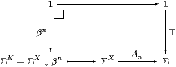
Proof The equation Anβn ⇔ ⊤ says that the square commutes. Any test map φ:Γ→ΣX↓βn that (together with !:Γ→1) also makes a square commute must satisfy Γ⊢ Anφ⇔⊤ and Γ⊢φ≤βn , but then φ=βn by the previous result. Hence the square is a pullback, whilst βn=⊤ΣK, so the lower composite is ∀K, making K compact. ▫
The following jargon will be useful:
Definition 6.6
An effective basis (βn,An) for an object X is called
| β0=λ x.⊥ and A0=λφ.⊤ |
| βn+m = βn∨βm and An+m = An∧ Am; |
| βn⋆ m = βn∧βm An ≤ An⋆ m and Am ≤ An⋆ m, |
Any effective basis can be “up-graded” to a lattice basis by formally adding unions and intersections (Lemma 8.4ff). It can be made into a filter ∨-basis instead (Remark 17.6). Some of the other terminology is only applicable in special situations: if A1⊤⇔⊤ then the object is compact, with ∀X=A1, whilst a sober topological space has a prime basis iff it is a continuous dcpo with the Scott topology (Theorem 12.11). Even when the intersection of two compact subobjects is compact, there is nothing to make An⋆ m correspond to it, but we shall rectify this in Proposition 12.14.
Examples 6.7 Let N be an overt discrete object. Then
| βn ≡ |
| ≡ λ x.(x=N n) and An ≡ ηN(n) ≡ λφ.φ n, |
| Bℓ≡ λξ.∀ m∈ℓ.ξ m and Aℓ≡ λ Φ.Φ(λ m.m∈ℓ), |
We devote the remainder of this section to showing that every locally compact sober space or locale has an effective basis in our sense. We start with traditional topology.
Proposition 6.8
Any locally compact sober space has a filter basis.
Proof Definitions 1.1 and 6 provide families (Kn) and (Un) of compact and open subspaces such that
| for each open V⊂ X, V = ⋃ {Un ∣ Kn ⊂ V}. |
As the subspace Kn is compact, Remark 5.6 defines An:ΣX→Σ such that Kn⊂ V iff Anφ⇔⊤, where βn and φ:ΣX classify Un and V⊂ X, so φ = ∃ n.Anφ∧βn. ▫
Notice how the basis decomposition “short changes” us, for individual basis elements: we “pay” Kn⊂ V but only receive Un⊂ Kn as a contribution to the union. Nevertheless, the interpolation property (Lemma 1.2) ensures that we get our money back in the end.
In many examples, Un may be chosen to be interior of Kn, and Kn the closure of Un. However, this may not be possible if we require an ∨-basis. For example, such a basis for ℝ would have as one of its members a pair of touching intervals, (0,1)∪(1,2), which is not the interior of [0,1]∪[1,2].
Remark 6.9 It is difficult to identify a substantive
Theorem by way of a converse to this in traditional topology,
since the λ-calculus can only by interpreted in topological spaces
if they are already locally compact, and therefore have effective bases.
Nevertheless, we can show that a filter basis (βn,An)
can only arise in the way that we have just described.
By Lemma 5.16, each An corresponds to some compact saturated subspace Kn, where
| (Kn⊂ V) ⇔ Anφ =⇒(Un⊂ V), |
βn and φ being the classifiers for Un and V as usual. Since Kn=⋂↓{V ∣ Kn⊂ V}, we must have Un⊂ Kn. Then, given x∈ V, so φ x⇔⊤, the basis decomposition φ x⇔∃ n.Anφ∧βn x, means that x∈ Un⊂ Kn⊂ V, as in Definition 1.1. ▫
Example 6.10 The closed real unit interval has a filter
∧-basis with
|
where є,δ>0 and q are rational, and we re-deploy the interval notation of Example 1.4 in our λ-calculus. We also write <q±δ> for a variable that ranges over the codes, as opposed to the open (q±δ) and compact [q±δ] intervals that it names. The imposed order is given by comparison of the radii є or δ.
Proof Let x∈ U⊂[0,1]; then, for some є> 0, ∀ y.|x−y|<є⇒ y∈ U. So with δ≡1/2є, and q rational such that |x−q|<δ,
| ∀ y. |
| ⇒ y∈ U ∧ x∈ |
| , |
which is ∃<q±δ>.Aq±δφ∧βq±δx in our notation. ▫
Example 6.11
Recall that any compact Hausdorff space X has a stronger property
called regularity: if C⊂ X is closed with x∉ C
then there are x∈ U⋔ V⊃ C with U,V⊂ X open and
disjoint.
Writing K=X∖ V and W=X∖ C for the complementary
compact and open subspaces, this says that given x∈ W,
we can find x∈ U⊂ K⊂ W, as in Definition 1.1.
Let (βn,γn) classify a sufficient computable family
(Un⋔ Vn) of disjoint open pairs,
and put An≡λφ.∀ x.φ x∨γn x,
which corresponds to the compact complement of Vn
(Proposition 5.11).
Then (βn,An) is a filter basis for X.
It is a lattice basis if the families (βn) and (γn)
are sublattices, with γ0=⊤, γ1=⊥,
γn+m=γn∧γm and
γn⋆ m=γn∨γm. ▫
Remark 6.12 In these idioms of topology, where we say that there
“exists” an open or compact subobject within certain bounds,
that subobject may typically be chosen to be basic,
and the existential quantifier in the assertion ranges over
the set (overt discrete object) N of indices for the basis,
rather than over the topology ΣX itself.
For example, this is the case with the Wilker property in
Lemmas 1.10 and 2.7.
Now we turn to locale theory.
Proposition 6.13 Any locally compact locale has a lattice
basis.
Proof The localic definition is that the frame L be a distributive continuous lattice (Definition 3), so
| for all φ∈ L, φ = ⋁ {β∈ L ∣ β≪φ}, |
and by Example 5.12, ↑β≡{φ ∣ β≪φ} is classified by some A:ΣL.
This means that there is a basis decomposition
| φ = ∃ n. βn ∧ Anφ, where An ≡ λφ.(βn≪φ), |
so (βn,An) is a lattice basis.
Recall, however, from Remark 3.9 that we must consider this basis to be indexed by the underlying set, |L|, of the frame L. Thus N≡|L|, whilst β(−):N→ L is the couniversal map from an overt discrete object N to L.
In fact it is enough for the image of N to generate L under directed joins (Definition 2.3). There is no need for N to be the couniversal way of doing this, and so no need for the underlying set functor |−|. ▫
Remark 6.14
The first part of the converse to this is Lemma 6.5,
but with the relative notion ≪ in place of compactness itself:
if Anφ⇔⊤ then βn≪φ
in the sense of Definition 2.
For suppose that φ≤⋁s↑θs, so
⊤ ⇔ Anφ ⇒ An⋁s↑θs
⇔ ⋁s↑ Anθs.
Then5
Anθs⇔⊤ for some s,
so βn≤θs by Lemma 6.4.
Now suppose that a locale carries an effective basis in our sense. Then
| φ = ∃ n.Anφ∧βn ≡ ⋁{βn ∣ Anφ} ≤ ⋁↑{βn ∣ βn≪φ} ≤ φ, |
in which the second join is directed, by Lemma 2.6. Hence the frame L is continuous. ▫
Remark 6.15
Notice that βm≤βn does not
imply any relationship between n,m∈ N,
because the function β(−):N→ L need not be injective.
This is the reason why An need not be exactly λφ.βn≪φ,
cf. Remark 1.8.
Proposition 6.16
A locale is stably locally compact iff it has a lattice
filter basis.
Proof [⇒] Let An=λφ.βn≪φ as before. [⇐] As we have an ∨-basis, the basis expansion is a directed join, to which we may apply the definition of βm≪φ. In this case there is some n with βm≤βn and Anφ⇔⊤, so βm≪⊤. Also, if βm≪φ and βm≪ψ then, for some p, q,
| βm≤βp, βm≤βq, Apφ⇔⊤ and Aqψ⇔⊤, |
so βm≤βp∧βq≡βp⋆ q. As we have a filter ∧-basis, Ap⋆ qφ∧ Ap⋆ qψ⇔ Ap⋆ q(φ∧ψ)⇔⊤. Hence, with n=p⋆ q, βm≤βn and An(φ∧ψ)⇔⊤, so βm≪φ∧ψ. ▫
Remark 6.17
In summary, the dual basis Anφ essentially says that
there is a compact subobject Kn lying between βn and φ,
but Kn seems to play no actual role itself,
and the localic definition in terms of ≪ makes it redundant,
cf. Proposition 2.2.
Nevertheless, each definition actually has its technical advantages:
Effective bases in our sense can be made to behave in either fashion, though we shall only consider lattice bases (cf. the localic situation) in this paper (Remark 17.6 sketches how filter bases may be obtained). Stably locally compact objects have lattice filter bases, whose properties will be improved in Proposition 12.14 to take advantage of the intersections of compact subobjects.