


We promised to translate each step of the logical development into topological language, but we haven’t done this since the end of Section 7. We shall now show how the “coding” provides the link between the classical and computational models (Remark 3.1), and then how abstract matrices themselves describe exact computation for the reals and locally compact objects in general.
Remark 17.1 On the one hand, we know from
the classical proof for LKSp in
Theorem A 5.12 and the intuitionistic one for LKLoc in
Theorem B 3.11 that these categories are models of the calculus in
Sections 3–4,
i.e. that there are interpretation functors ⟦−⟧:S→LKSp
and ⟦−⟧:S→LKLoc.
In the light of Theorem 8.11,
that every object of S is a Σ-split subobject of Σℕ,
the converse part of Theorem 7.14
provides another proof in the localic setting.
In this paper we have sought the “inverse” of this functor. Since the classical models are of course richer, they have to be constrained in order to obtain something equivalent to the computational one (Remark 3.1). This constraint was in the form of a computable basis, as in Definitions 1.5 and 2.3. Nevertheless, as we saw in the case of ℝ (Example 1.4), such bases may already be familiar to us from traditional considerations.
There is no need to verify the consistency conditions that we set out in Sections 11 and 14. They follow automatically from the existence of the classical space, which serves as a reference as in Remark 1.7. So long as ⋆, + and ≺≺ are defined by programs, which can be translated into our λ-calculus, we already have an abstract basis.
Examples 17.2
At this point let us recall the various ways in which
a lattice basis can be defined on a locally compact sober space or locale.
| βℓx ≡ ∀ n∈ℓ.x ∈ Un and Aℓφ ≡ ∃ n∈ℓ.Kn⊂ V, |
| ℓ≺≺ ℓ′ ⇔ ∃ n∈ℓ.∀ m∈ℓ′.Kn⊂ Um, |
Remark 17.3 Section 14 showed that the abstract basis is
inter-definable with the nucleus E. These are interpreted both in
the computational model S and in the classical ones LKSp and
LKLoc. This means that the idempotent ⟦E⟧ on
ΥKℕ is the one that defines the Σ-split
embedding of the original space in ℘(ℕ),
as in Theorems 7.8 and 7.14.
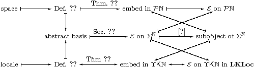
Hence any classically defined locally compact sober space or locale that has a computable basis may be “imported” into abstract Stone duality as an object, whose interpretation in the classical model is homeomorphic to the given space. Summing this up diagrammatically,
Remark 17.4 Having fixed computational bases for two classically defined
spaces or locales, X and Y, we may look at continuous functions
f:X→ Y.
By the basis property, any such map is determined by the relation
| f Kn ⊂ Vm |
as n and m range over the bases for X and Y respectively. If this relation is recursively enumerable (Definition 1.6) then the corresponding program may be translated into our λ-calculus. Just as we saw for abstract bases, the resulting term satisfies Definition 16.12 for an abstract matrix, because its interpretation agrees with a continuous function. Between the objects whose denotations are X and Y there is therefore a term whose denotation is f.
In particular, computationally equivalent bases for the same space give rise to an isomorphism between the objects of S. In the case of morphisms, extensionally equivalent terms give rise to the same (f Kn⊂ Vm)-relations, and therefore to the same continuous functions. However, programs may be extensionally equivalent for some deep mathematical reason, or as a result of the stronger logical principles in the classical situation, without being provably equivalent within our calculus. This is the reason why we required the computable aspects of the definitions in the Introduction to be accompanied by actual programs.
This completes the proof of our main result:
Theorem 17.5 Abstract Stone duality, i.e. the free model S
of the axioms in Sections 3 and 4,
is equivalent to the category of computably based locally compact locales
and computably continuous functions. ▫
Remark 17.6
An obvious lacuna in this result arises from the difference
between sober spaces and locales: we are relying on the axiom of
choice within the classical models to say that the two are the same.
Recall [Joh82, Theorem VII 4.3]
that, using excluded middle, the crucial requirement is to find,
for any φ≰ψ:L in a distributive continuous lattice,
For stage (a), we would like to show, more generally, that every object (which we know carries a lattice basis) also has a filter ∨-basis. The idea, due to Jimmie Lawson [GHK++80, §I 3.3], is to iterate the interpolation property [G–]. This can be shown with the aid of a weaker choice principle that merely extracts a total function from a non-deterministic one.
For stage (b), since any space has a ℕ-indexed lattice basis, we only need to consider Σℕ, and not general distributive continuous lattices. The filter A provides a rounded filter (semilattice homomorphism) ξ0:Σℕ such that Iφξ⇔⊤ but Iψξ⇔⊥, which we enlarge to a rounded lattice homomorphism ξ (Lemmas 15.2ff) with the same values on φ and ψ. To do this, we may replace Zorn’s Lemma by an argument that uses excluded middle but not Choice: we build up ξ from ξ0 by adding each number 0, 1, 2, ... in turn if it generates a proper filter. ▫
Remark 17.7 Let’s review what we’ve achieved by way of
a type theory for topology.
Remark 17.8 Let us consider
the computational meaning of the matrix Hnm
when H≡Σf for some continuous function f:ℝ→ℝ.
In order to have a lattice basis,
the indices n and m must range over (finite) unions of intervals,
although by Lemma 16.3, n need only denote a single closed interval.
The matrix therefore encodes the predicate
| f[x0±δ] ⊂ ⋃j(yj±єj), |
as an ASD term of type Σ, the union being finite. Suppose that we have a real input value x that we know to lie in the interval [x0±δ], and we require f(x) to within є.
We substitute the rational values x0, δ and єj≡є in the predicate, leaving (yj) indeterminate. Recall from Remark 3.5 and Section t ha t any such term may be translated into a λ-Prolog program. Such a program permits substitution of values for any subset of the free variables, and is executed by resolving unification problems, which result in values of (or at least constraints on) the remaining variables. In this case, we obtain (nondeterministically) some finite set (yj).
In the language of real analysis, we are seeking to cover the compact interval f[x0±δ] with (finitely many) open intervals of size є, centred on the yj. The Wilker property (Lemma 16.11) then provides
| [x0±δ] ⊂ ⋃j(xj±δ′) with f[xj±δ′] ⊂ (yj±є). |
Responsibility now passes back to the supplier of the input value x to choose which of the xj is nearest, and the corresponding yj is the required approximation to the result f(x). This discussion is taken up again in [I, J]. ▫
Remark 17.9 This illustrates the way in which we would expect to use
abstract Stone duality for computations with objects such as ℝ
that we regard, from a mathematical point of view, as “base types”
(though of course only 1, ℕ and Σ are
actually base types of our λ-calculus).
Where higher types, such as continuous or differentiable function-spaces,
can be shown to be locally compact, they too have bases and matrices,
but it would be an example of the mis-use of normalisation theorems
(Remark 8.12) to insist on reducing everything to matrix form.
We would expect to use higher-type λ-terms of our calculus
to encode higher-order features of analysis, for example in the
calculus of variations.
Of course, much preliminary work with ℝ itself needs to be
done before we see what can be done in such subjects
[I, J].
Remark 17.10 The manipulations that we have done since introducing the
abstract way-below relation have all required lattice bases.
The naturally occurring basis on an object such as ℝ,
on the other hand, is often just an ∧-basis.
This didn’t matter in Sections 14–16,
as they were only concerned with the theoretical issue
of the consistency of the abstract basis.
We have just seen, however, that the “matrices” in Section 16
encapsulate actual computation, in which the base types are those
of the indices of the bases. The lists used in
Lemma 8.4 would then be a serious burden.
There is a technical issue here that is intrinsic to topology. In locale theory, which is based on an algebraic theory of finite meets distributing over arbitrary unions of “opens”, it is often necessary to specify when two such expressions are equal, which may be reduced to the question of when an intersection is contained in a union of intersections. This coverage relation is an important part of the technology of locale theory [Joh82, Section II 2.12], whilst it was chosen as the focus of the axiomatisation of Formal Topology.
Remark 17.11 The question of whether, using abstract Stone duality,
we can develop a technically more usable approach than these
warrants separate investigation, led by the examples.
Since, in a locally compact object,
we may consider coverages of compact subobjects,
the covering families of open subobjects need only be finite.
Jung, Kegelmann and Moshier have exploited this idea to develop a
Gentzen-style sequent calculus [JKM99].
As this finiteness comes automatically, maybe we don’t need to force it by using lists. To put this another way, as the lists act disjunctively, we represent them by their membership predicates (Remark 8.5). That is, we replace the matrix Hmn with the predicate
| m:M, ξ:ΣN ⊢ Am· H(λ y.∃ n.ξ n∧βn y):Σ, |
where N need no longer have +. In Remark 17.8 above, we could add the constraint that ξ only admits intervals of size <є.
Remark 17.12
Another striking feature of the matrix description is that it
reduces the topological theory to an entirely discrete one.
The latter may be expressed in an arithmetic universe,
which is a category with finite limits, stable disjoint coproducts,
stable effective quotients of equivalence relations and a List functor
[E].
Once again, we need to see this normalisation theorem in reverse. It appears that any arithmetic universe may conversely be embedded as the full subcategory of overt discrete objects in a model of abstract Stone duality. Example 4 shows that we can do this by modelling a much simpler structure than that of abstract bases and matrices for general locally compact spaces. The differences in logical strength amongst models of ASD are therefore measured by the overt discrete objects that they contain.
Such a construction would enable topological, domain-theoretic and λ-calculus reasoning to be applied to problems in discrete algebra and logic. Topologically, it would strongly vindicate Marshall Stone’s dictum, always topologise, whilst computationally it would provide continuation-passing translations of discrete problems, and of type theories for inductive types.